
Beer Lambert Law Calculator
A = ε l c, solved for whichever term you are missing. This Beer Lambert law calculator converts absorbance to concentration (and back) with any molar or specific absorptivity and path length, turns transmittance into absorbance, builds a calibration curve by least squares and reads unknowns off it, corrects for dilution and the linear range, and handles multi-wavelength two-component mixtures.
✓ Trusted by analytical, biochemistry & environmental labsSolve the Beer-Lambert Equation for Any Variable
Leave exactly one of A, ε, l, c blank (or choose it below) and the Beer Lambert law calculator solves for it. ε may be a molar absorptivity (M⁻¹cm⁻¹), a specific absorptivity (L g⁻¹ cm⁻¹ or the A1%1cm value), and concentration can be returned in M, mM, µM or mg/mL if you give the molar mass.
Transmittance, Absorbance and the Fraction of Light Absorbed
A = −log₁₀(T) = 2 − log₁₀(%T). Enter %T, T or A and the Beer Lambert law calculator returns the others, the fraction absorbed, and the concentration if you also give ε and l; it also shows how much a 1 % transmittance error moves the answer at your absorbance (why 0.1–1.0 A is the sweet spot).
Calibration Curve: Least-Squares Fit and Unknowns
Paste standards as concentration, absorbance per line (any concentration unit). The Beer Lambert law calculator fits A = m·c + b (and the through-origin fit), reports slope, intercept, R², the effective ε and the LOD/LOQ from the residuals, then converts your unknown absorbances into concentrations with a dilution factor.
Dilute a Sample into the Linear Range
Absorbance above ~1.5 (and readings below ~0.05) are unreliable. Give the measured absorbance (even an off-scale estimate), the target absorbance window and the sample volume; the Beer Lambert law calculator recommends a dilution factor, the volumes to pipette, and the original concentration once you supply ε or a calibration slope.
Two-Component Mixture from Two Wavelengths
Absorbances are additive: Aλ1 = εX,1 l cX + εY,1 l cY and likewise at λ2. Enter the four molar absorptivities and the two absorbances; the Beer Lambert law calculator solves the 2 × 2 system for both concentrations and reports the condition of the system (how well-separated the spectra are).
🕘 Recent calculations
- No calculations yet — your last 10 results will appear here.
Formulas: A = ε l c (ε in M⁻¹cm⁻¹, l in cm, c in mol/L) · specific absorptivity a (L g⁻¹cm⁻¹) = ε / M; A1%1cm = 10 a · A = −log₁₀ T = 2 − log₁₀(%T); T = 10⁻A · fraction absorbed = 1 − T · least squares: m = Σ(x−x̄)(y−ȳ)/Σ(x−x̄)², b = ȳ − m x̄; R² = 1 − SSres/SStot; LOD = 3.3 sy/x/m, LOQ = 10 sy/x/m · unknown c = (A − b)/m × dilution factor · two components: solve A₁ = εX1lcX + εY1lcY, A₂ = εX2lcX + εY2lcY by Cramer's rule · Beer-Lambert holds for dilute (< ~10 mM), non-scattering, monochromatic conditions; keep 0.1 < A < 1.0 for best precision.
A Beer Lambert law calculator solves A = εlc — absorbance equals molar absorptivity times path length times concentration — for whichever of the four quantities you do not know, and handles the practical questions that surround every spectrophotometer: what absorbance a transmittance reading corresponds to, how to fit a calibration curve and read unknowns from it, how far to dilute a sample that reads off scale, and how to resolve two absorbing species from readings at two wavelengths.
The free Beer Lambert law calculator on this page has five modes: a solver for A, ε, l or c in molar, specific (per gram) or A1% absorptivity units with mg/mL and µM outputs; transmittance to absorbance with the error sensitivity at your reading; a least-squares calibration curve with slope, intercept, R², LOD, LOQ and unknown read-back including a dilution factor; a dilution planner that brings any absorbance into the 0.1–1.0 window with the volumes to pipette; and a two-component mixture solver using Cramer’s rule with a conditioning check. Every result shows the working, a table and a chart.
Below the tool you will find the law and its derivation, units and the three kinds of absorptivity, the transmittance relationship and why 0.1–1.0 A is the sweet spot, calibration statistics, deviations from linearity, worked examples for NADH, DNA, proteins and permanganate, a table of common molar absorptivities, ten practice problems, a checklist and the questions readers ask most about the Beer Lambert law calculator.
Key Takeaway
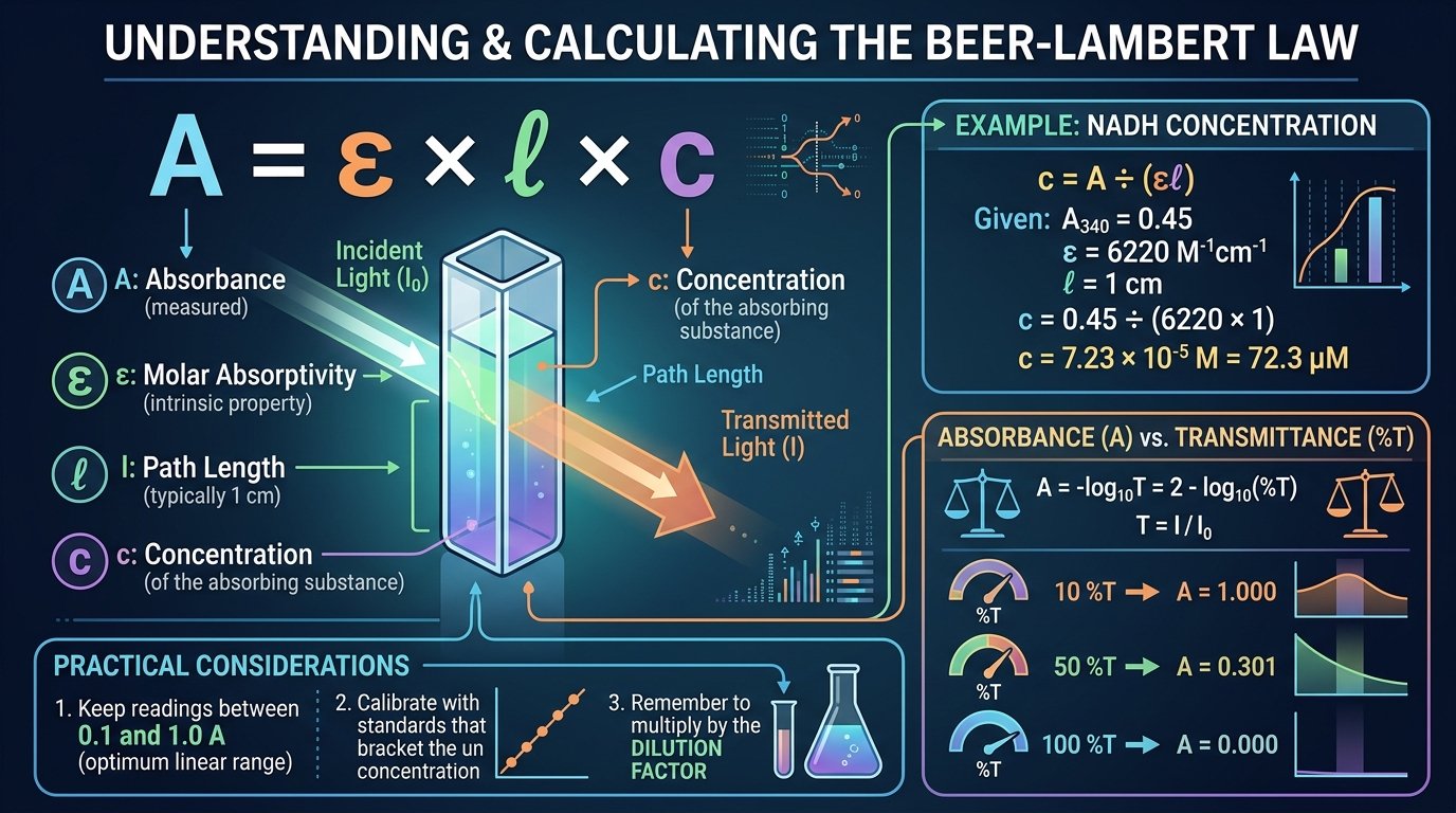
A = ε × l × c, so c = A ÷ (εl). NADH with A340 = 0.45 in a 1 cm cuvette (ε = 6220 M−1cm−1) is 72.3 µM. Absorbance and transmittance are linked by A = −log10T = 2 − log10(%T): 10 %T is A = 1.000, 50 %T is 0.301. Keep readings between 0.1 and 1.0 A, calibrate with standards that bracket the unknown, and multiply by the dilution factor. The Beer Lambert law calculator above does all of this with the steps shown.
📑 Table of Contents (click to expand)
- What Is a Beer Lambert Law Calculator?
- How to Use the Beer Lambert Law Calculator
- The Five Modes Explained
- The Law, Its Derivation and Its Units
- Worked Example: NADH at 340 nm
- Transmittance, Absorbance and the 0.1–1.0 Window
- Calibration Curves: Least Squares, R², LOD and LOQ
- More Worked Examples
- The Three Kinds of Absorptivity
- When the Law Fails: Deviations From Linearity
- Two Components, Two Wavelengths
- Diluting Into the Linear Range
- Kinetic Assays: From ΔA per Minute to Rates
- Reference Table: Molar Absorptivities
- Visualising Absorbance
- Who Uses a Beer Lambert Law Calculator
- Full Walkthrough: Phosphate by the Molybdenum-Blue Method
- A Short History of the Beer-Lambert Law
- Limits and Assumptions
- Practice Problems With Answers
- Tips for Accurate Results
- Common Mistakes
- How This Beer Lambert Law Calculator Is Different
- Where the Numbers Come From
- Checklist
- Frequently Asked Questions
- 10 Facts Worth Knowing
- Final Thoughts
What Is a Beer Lambert Law Calculator?
The Beer-Lambert law (also Beer’s law or the Beer-Lambert-Bouguer law) states that the absorbance of a solution is directly proportional to the concentration of the absorbing species and to the distance the light travels through it. Written A = εlc, it is the working equation of absorption spectrophotometry: measure A, know ε and l, and the concentration follows by division. A Beer Lambert law calculator does that division — and the multiplications and rearrangements for the other unknowns — with the units handled correctly, then extends it to the transmittance scale, to calibration curves, to dilution planning and to mixtures.
The quantities the Beer Lambert law calculator works with: A is absorbance, dimensionless, defined as log10(I0/I); ε is the molar absorptivity (molar extinction coefficient) in L mol−1 cm−1, a property of the substance at a given wavelength and solvent; l is the path length in cm, 1.00 cm for a standard cuvette; c is the molar concentration. Because ε can also be quoted per gram (specific absorptivity, L g−1 cm−1) or per 1 % solution (A1%1cm, used in pharmacopoeias), the Beer Lambert law calculator accepts all three and converts between them when the molar mass is supplied.
Rearrangements
c = A / (ε l) · ε = A / (l c) · l = A / (ε c) · A = ε l c
Specific absorptivity a = ε / M; A1% = 10 a; c (mg/mL) = A / (a l). The Beer Lambert law calculator solves whichever form your data are in.
How to Use the Beer Lambert Law Calculator
- Pick the mode. Solve A = εlc for any single unknown; Transmittance to convert %T or T; Calibration curve to fit standards and read unknowns; Dilution when a reading is off scale; Mixture for two species at two wavelengths.
- Enter the known values with units. ε as M−1cm−1, mM−1cm−1, L g−1cm−1 or A1%; concentration in M, mM, µM, mg/mL or µg/mL; path in cm (0.1 for a 1-mm cell). Add the molar mass when crossing between molar and mass units.
- Press Solve. The Beer Lambert law calculator prints the unknown in blue, the concentration in both molar and mass units when possible, the transmittance and absorbed fraction, a warning if A is outside 0.1–1.0, the steps, a table and a chart.
- For calibration, paste standards as
concentration, absorbancelines and unknown absorbances; set the dilution factor; the fit, statistics and unknown concentrations appear together. - Copy, download, print or share; each mode has its own Reset and the history box keeps ten results.
The chips load NADH at 340 nm, BSA at 280 nm, dsDNA at 260 nm, a specific-absorptivity case, %T conversions, a permanganate calibration series, an off-scale dilution and the chlorophyll a/b mixture, so the Beer Lambert law calculator’s output is visible before you type.
The Five Modes Explained
Mode 1 — Solve. Choose the unknown, supply the other three. Handles molar and specific absorptivities, converts concentrations through the molar mass, reports T and the absorbed fraction, warns above 1.5 A and below 0.05 A, and charts A for 0.25×, 0.5×, 1× and 2× the concentration.
Mode 2 — Transmittance. %T, T or A in; the other two out; blank correction for a non-100 % reference; concentration if ε and l are given; and the change in A per 1 %T reading error at your value — the quantitative reason to work near A = 0.43.
Mode 3 — Calibration curve. Least-squares slope, intercept and their standard errors, R², sy/x, the through-origin slope, LOD = 3.3 s/m and LOQ = 10 s/m, ε from the slope when the units allow, residuals for every standard, and unknowns converted with a dilution factor and flagged if above the top standard or below LOQ.
Mode 4 — Dilution. A measured (or estimated off-scale) absorbance, a target window and a final volume; the Beer Lambert law calculator picks a convenient factor, gives sample and solvent volumes, expected A, the total dilution including any already applied, and the original concentration if ε or a slope is supplied. Recognises samples that are too weak and suggests a longer path.
Mode 5 — Two-component mixture. Four absorptivities, two absorbances, path length; solves the 2 × 2 system, back-checks, shows each species’ share at each wavelength and reports the condition number so you know whether the wavelengths were well chosen.
The Law, Its Derivation and Its Units
To see where the Beer Lambert law calculator’s equation comes from, consider light of intensity I passing through a thin slab of solution of thickness dx. The fraction absorbed is proportional to the number of absorbing molecules in the slab, i.e. to c·dx: dI/I = −k c dx. Integrating from 0 to l gives ln(I0/I) = k c l, and converting to base-10 logarithms, log10(I0/I) = A = ε c l with ε = k/2.303. Lambert (1760) stated the dependence on path length, Beer (1852) the dependence on concentration; Bouguer had described the path-length law in 1729.
A = log10(I0/I) = ε l c
ε in L mol−1 cm−1, l in cm, c in mol L−1; A dimensionless. Absorbances of independent species add: Atotal = Σ εi l ci.
The units must multiply to a pure number, which is the check the Beer Lambert law calculator performs silently: a molar ε needs a molar concentration, a specific absorptivity needs g/L, and an A1% value (the absorbance of a 1 g per 100 mL solution in 1 cm) is ten times the specific absorptivity. Molar absorptivity ranges from below 1 for weak d-d transitions (Cu2+ at 800 nm, ε ≈ 12) to over 105 for strongly allowed π→π* transitions in dyes; it depends on wavelength, solvent, pH and temperature, so it must be quoted with all of them.
Worked Example: NADH at 340 nm
An enzyme assay follows NADH, whose molar absorptivity at 340 nm is 6220 M−1cm−1. The cuvette reads A = 0.450 against a buffer blank in a 1.00 cm cell.
- Rearrange. c = A / (ε l).
- Substitute. c = 0.450 / (6220 × 1.00) = 7.23 × 10⁻⁵ mol/L = 72.3 µM.
- Mass units. With M = 663.4 g/mol (disodium salt), 72.3 µM × 663.4 = 48.0 mg/L = 48.0 µg/mL.
- Check. T = 10−0.45 = 35.5 %; 64.5 % of the light was absorbed; A is within 0.1–1.0. ✓
In a kinetic assay the same Beer Lambert law calculator arithmetic converts a rate of change of absorbance into a rate of change of concentration: ΔA/min ÷ 6220 = Δc/min in M/min, so 0.062 A/min is 10 µM/min. The Beer Lambert law calculator’s solver handles the per-minute case as an ordinary absorbance; for mass-based ε values (proteins, nucleic acids) it converts through the molar mass, as the next sections show.
Transmittance, Absorbance and the 0.1–1.0 Window
Spectrophotometers measure transmitted intensity; absorbance — what the Beer Lambert law calculator works in — is computed from it. T = I/I0, %T = 100 T, and A = −log10 T = 2 − log10(%T). The scale is logarithmic: A = 1 means 10 % transmitted (90 % absorbed), A = 2 means 1 %, A = 3 means 0.1 %. The Beer Lambert law calculator converts in any direction and, when a blank does not read exactly 100 %T, corrects against it.
| %T | A | Absorbed | Relative error in c per 1 %T error |
|---|---|---|---|
| 90 | 0.046 | 10 % | 10.5 % |
| 79.4 | 0.100 | 21 % | 5.5 % |
| 36.8 | 0.434 | 63 % | 2.7 % (minimum) |
| 10 | 1.000 | 90 % | 4.3 % |
| 3.16 | 1.500 | 96.8 % | 9.2 % |
| 1 | 2.000 | 99 % | 21.7 % |
The last column is why textbooks say to keep A between roughly 0.1 and 1.0: the relative error in concentration from a fixed error in transmittance is smallest at A = 0.434 (T = 36.8 %) and rises steeply on both sides. Modern instruments have smaller and more complex error functions, and the upper limit is set less by photometric noise than by stray light, which flattens the response above about 1.5–2 A. The Beer Lambert law calculator’s mode 2 evaluates the error term at your reading and its mode 4 plans a dilution back into the window.
Calibration Curves: Least Squares, R², LOD and LOQ
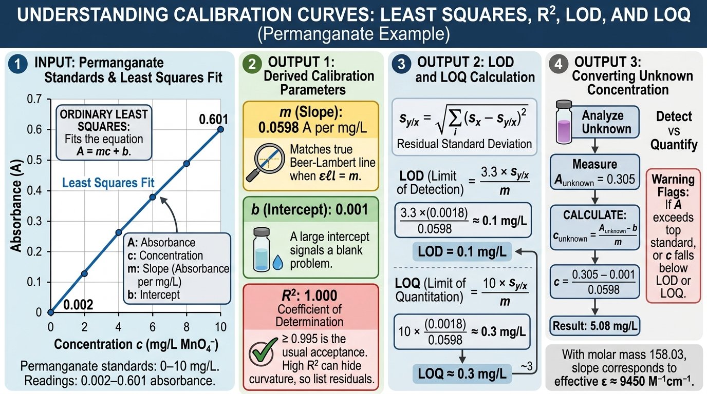
When ε is unknown, uncertain, or the method is not strictly a Beer-Lambert measurement, the Beer Lambert law calculator switches to calibration (colorimetric assays such as Bradford, Griess or phosphate-molybdate), the concentration is read from a calibration curve of absorbance against standards. The Beer Lambert law calculator fits A = m·c + b by ordinary least squares and reports:
- Slope m (absorbance per concentration unit) — equal to εl when the curve is a true Beer-Lambert line — and its standard error.
- Intercept b and its standard error; a large intercept signals a blank problem.
- R², the fraction of variance explained; ≥ 0.995 is the usual acceptance, but curvature at the top standard can hide behind a high R², so the residuals are listed too.
- sy/x, the residual standard deviation, and from it LOD = 3.3 sy/x/m and LOQ = 10 sy/x/m (ICH Q2 calibration-curve approach).
- Unknowns: c = (A − b)/m × dilution factor, flagged when A exceeds the top standard (extrapolation) or c falls below LOQ or LOD.
For permanganate standards of 0–10 mg/L reading 0.002–0.601, the tool returns m = 0.0598 A per mg/L, b = 0.001, R² = 1.000, LOD 0.1 mg/L, and converts an unknown of 0.305 to 5.08 mg/L; with the molar mass (158.03) the slope corresponds to an effective ε of about 9450 M−1cm−1 for this illustrative data set (the accepted value at 525 nm is about 2400, so real permanganate standards would give a shallower slope). Good calibration practice — a blank, five or six levels, the unknown bracketed, no extrapolation — is spelled out in the tool’s notes. For preparing the standards themselves see the dilution calculator and serial dilution calculator.
More Worked Examples
Example 1 — BSA at 280 nm
ε = 43 824 M−1cm−1, M = 66 430; A = 0.52, l = 1 cm: c = 0.52 / 43 824 = 11.9 µM = 0.788 mg/mL. Equivalently ε0.1% = 43 824 / 66 430 = 0.66 and 0.52 / 0.66 = 0.79 mg/mL.
Example 2 — dsDNA at 260 nm
Specific absorptivity 20 L g−1cm−1 (A260 = 1 for 50 µg/mL); A = 0.8 → 0.8 / 20 = 0.04 g/L = 40 µg/mL.
Example 3 — Pharmacopoeial A1%
A(1 %, 1 cm) = 24 means a = 2.4 L g−1cm−1; A = 0.9 → 0.9 / 2.4 = 0.375 g/L = 375 µg/mL.
Example 4 — Finding ε
A 25 µM solution reads 0.72 in 1 cm: ε = 0.72 / (1 × 25 × 10−6) = 28 800 M−1cm−1.
Example 5 — Off-scale sample
A reads 2.8 (unreliable). Target 0.2–0.8: dilute 1 : 4 (250 µL + 750 µL) for an expected 0.7; remeasure and multiply by 4. With ε = 6220 the original is about 450 µM.
The Three Kinds of Absorptivity
| Name | Symbol / units | Concentration unit | Conversion |
|---|---|---|---|
| Molar absorptivity | ε, L mol−1 cm−1 | mol/L | — |
| Specific absorptivity | a (or ε0.1%), L g−1 cm−1 = mL mg−1 cm−1 | g/L = mg/mL | a = ε / M |
| A(1 %, 1 cm) | A1%1cm, dL g−1 cm−1 | g per 100 mL | A1% = 10 a = 10 ε / M |
| mM absorptivity | mM−1 cm−1 | mmol/L | × 1000 = ε |
Biochemists mix these freely — “ε = 6.22 mM−1cm−1” for NADH, “ε0.1% = 0.66″ for BSA, “A1% = 24″ in a monograph — and a unit slip is a factor of 10, 1000 or the molar mass. The Beer Lambert law calculator takes each form explicitly and refuses to combine a per-gram absorptivity with a molar concentration until the molar mass is given, at which point it reports both. The protein-specific version of this arithmetic, with ε predicted from sequence, is in our protein concentration A280 calculator.
When the Law Fails: Deviations From Linearity
The equation in the Beer Lambert law calculator is a limiting law for dilute, homogeneous, non-scattering solutions measured with monochromatic light. Deviations arise from:
- Concentration above about 0.01 M, where solute molecules interact and the refractive index changes — real chemical deviations.
- Chemical equilibria — dimerisation of dyes, acid-base speciation with pH, complex formation — which change the absorbing species with concentration; isosbestic points and pH buffering are the remedies.
- Polychromatic light: a bandwidth wide relative to the absorption band gives negative curvature, because the strongly absorbed wavelengths are removed first. Measure at a maximum, where ε varies least.
- Stray light: a fixed fraction of unabsorbed light reaching the detector sets a ceiling on measurable A (0.1 % stray light caps A near 3 and bends the line above 2).
- Scattering by turbidity or aggregates, which raises apparent absorbance at all wavelengths; check a baseline at 320–350 nm for proteins.
- Fluorescence reaching the detector, which lowers apparent A.
Practically, the linear range is established by the calibration curve, and the Beer Lambert law calculator’s residual list and R² are where curvature shows up. If the top standards fall below the line, the range is too wide; drop them or dilute. For the molar-mass side of unit conversions the molarity calculator is the companion tool.
Two Components, Two Wavelengths
Because absorbances add, the Beer Lambert law calculator can resolve a mixture of two absorbing species from readings at two wavelengths if the molar absorptivities of both species at both wavelengths are known: A1 = εX1lcX + εY1lcY and A2 = εX2lcX + εY2lcY. The Beer Lambert law calculator solves the pair by Cramer’s rule, back-substitutes to check, and reports the condition number of the system — a measure of how much measurement error is amplified. Well-chosen wavelengths (each near one species’ maximum and the other’s minimum) give condition numbers near 1–3; poorly chosen ones give 20 or more and unreliable answers.
Classic applications loaded as chips in the Beer Lambert law calculator: chlorophyll a and b in 80 % acetone at 663 and 645 nm (Arnon’s equations are exactly this system); oxy- and deoxyhaemoglobin at 560 and 576 nm; NAD+ and NADH at 260 and 340 nm; Cr3+ and Co2+ in the teaching laboratory. With three or more species, more wavelengths and a least-squares fit are needed — the basis of multicomponent analysis in modern diode-array instruments.
Diluting Into the Linear Range
A reading above about 1.5 A cannot be trusted, and the Beer Lambert law calculator says so; and a reading of 3 or “OVER” is only a statement that the sample is dark. The right response is a dilution that brings the expected absorbance into the 0.1–1.0 window (or the range of your calibration standards), followed by a fresh measurement and multiplication by the dilution factor. The Beer Lambert law calculator’s mode 4 chooses a convenient factor aimed at the geometric centre of the window (√(0.2 × 0.8) = 0.4), gives the sample and solvent volumes for the cuvette volume you have, and keeps track of any dilution already applied so the final factor is right.
Two refinements the Beer Lambert law calculator notes: dilute in the same solvent as the blank, so the baseline is unchanged; and when the sample is too weak (A < 0.05), use a longer path (5 or 10 cm cells), concentrate the sample, choose a wavelength with a higher ε, or switch to a more sensitive method. The tool detects the weak case and lists those options instead of a dilution. For the general arithmetic of dilution factors see the dilution calculator.
Kinetic Assays: From ΔA per Minute to Rates
Enzyme assays follow absorbance over time, and the Beer Lambert law calculator serves them too: and the Beer-Lambert law converts a slope in absorbance units per minute into a rate in concentration per minute: Δc/Δt = (ΔA/Δt) / (εl). For NADH-linked dehydrogenases a slope of 0.0622 A/min in a 1 cm cuvette is 10 µM/min; multiplied by the cuvette volume (1 mL) it is 10 nmol/min, and divided by the enzyme mass it becomes the specific activity in units per milligram. The Beer Lambert law calculator’s solver accepts the slope as “A” and returns the rate as “c”, and the same unit discipline applies — a mM−1cm−1 absorptivity gives mM/min.
Two practical points the Beer Lambert law calculator cannot check for you: use the initial linear portion of the trace (before substrate depletion bends it), and keep the starting absorbance low enough that the whole trace stays under about 1.5 A. p-Nitrophenol (ε 18 000 at 405 nm, pH 10), NADH (6220 at 340 nm) and DTNB’s TNB anion (14 150 at 412 nm) are the workhorse chromophores; their absorptivities are pH-dependent, so the assay buffer’s pH must match the value quoted.
Reference Table: Molar Absorptivities
| Substance | λ (nm) | ε (M−1cm−1) | c for A = 0.5, 1 cm | Use |
|---|---|---|---|---|
| NADH / NADPH | 340 | 6 220 | 80 µM | Dehydrogenase assays |
| p-Nitrophenol (pH 10) | 405 | 18 000 | 28 µM | Phosphatase, ELISA |
| Tryptophan | 280 | 5 500 | 91 µM | Protein A280 |
| Tyrosine | 280 | 1 490 | 336 µM | Protein A280 |
| BSA | 280 | 43 824 | 11.4 µM (0.76 mg/mL) | Protein standard |
| dsDNA (per bp) | 260 | 13 200 (6600 per nt) | 25 µg/mL | Nucleic acid quantitation |
| KMnO4 | 525 | 2 400 | 208 µM | Teaching, COD |
| Cu2+(aq) | 810 | 12 | 42 mM | Weak d-d band |
| Fe(phen)32+ | 510 | 11 100 | 45 µM | Iron determination |
| Methylene blue | 664 | ~75 000 | 6.7 µM | Dye, photochemistry |
Values are typical literature figures at the stated wavelengths in the usual solvents; consult the source for your conditions. Each row converts to a concentration in the Beer Lambert law calculator with one line.
Visualising Absorbance
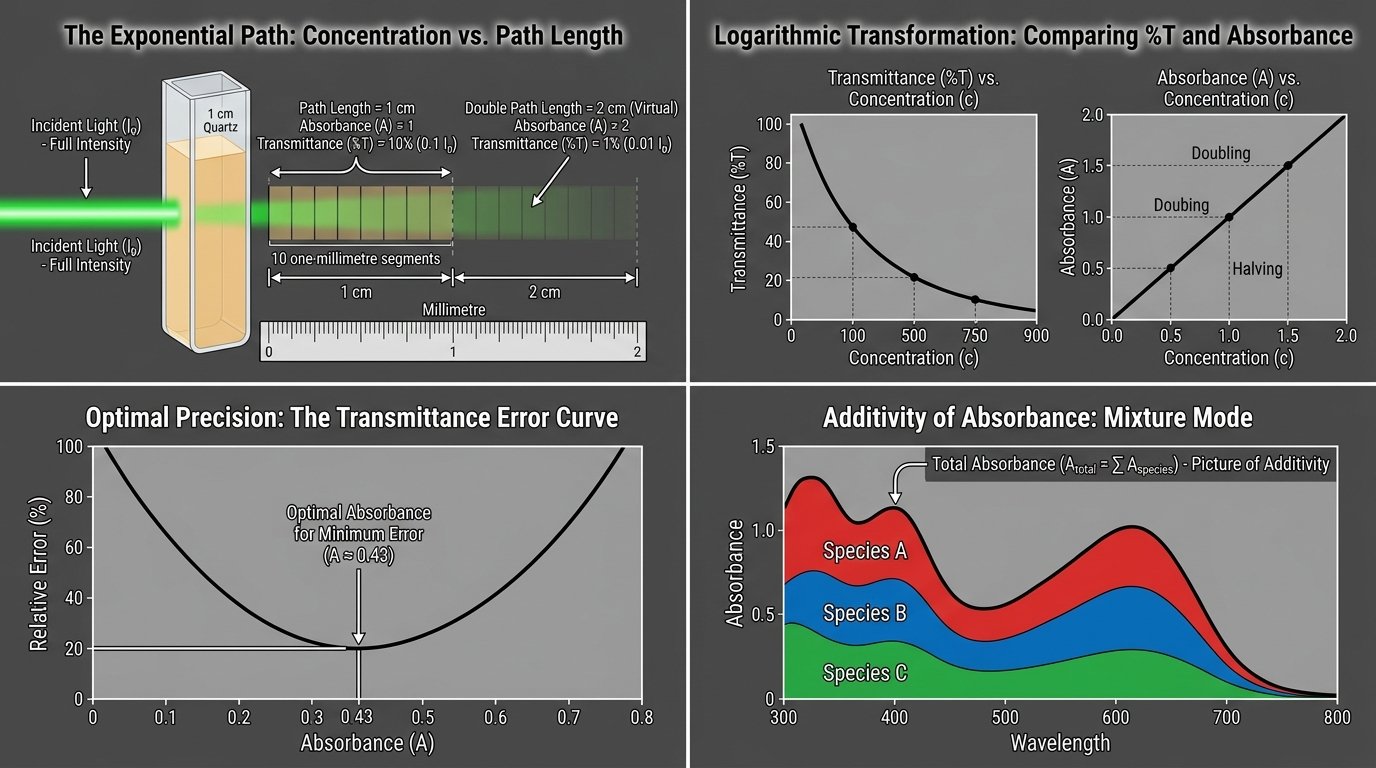
Picture the Beer Lambert law calculator’s cuvette: a beam enters at full intensity and losing a fixed fraction in every millimetre: after 1 cm of a solution with A = 1, one-tenth remains; after 2 cm, one-hundredth. Doubling the concentration has exactly the effect of doubling the path. That exponential decay of intensity is why absorbance — the logarithm — is the linear quantity, and why a plot of A against c is a straight line through the origin while a plot of %T against c is a curve.
The Beer Lambert law calculator’s charts reinforce this: the solver mode shows A doubling and halving with concentration, the transmittance mode shows the error curve with its minimum near A = 0.43, the calibration mode plots standards and unknowns side by side, and the mixture mode stacks each species’ contribution at each wavelength — a picture of additivity.
Who Uses a Beer Lambert Law Calculator
Biochemists quantify NADH, proteins, nucleic acids and enzyme rates. Analytical and environmental chemists run colorimetric methods for phosphate, nitrite, iron and chlorine with calibration curves. Pharmaceutical analysts apply A1% values from pharmacopoeial monographs. Clinical laboratories measure bilirubin, haemoglobin and enzyme activities photometrically. Plant scientists determine chlorophylls from two-wavelength equations. Students meet A = εlc in first-year chemistry and use it in every laboratory course after.
The Beer Lambert law calculator serves all of them by taking absorptivity in whatever form the source gives it, producing concentration in whatever unit the report needs, and making the statistics of a calibration curve as easy as the arithmetic of a single measurement.
Full Walkthrough: Phosphate by the Molybdenum-Blue Method
- Standards. 0, 1, 2, 5, 10 and 20 mg/L phosphate-P developed with molybdate/ascorbate; absorbances at 880 nm: 0.000, 0.052, 0.101, 0.255, 0.498, 0.960.
- Fit in the Beer Lambert law calculator’s mode 3: m = 0.0489 A per mg/L, b = 0.003, R² = 0.9998, sy/x = 0.006, LOD 0.4 mg/L, LOQ 1.2 mg/L. The 20 mg/L residual is slightly negative — the first hint of curvature.
- Unknowns, diluted 1 : 2 before colour development: A = 0.150, 0.720, 1.100. Read-back: 3.0, 14.7 and (flagged: above top standard) 22.4 mg/L × 2 = 6.0, 29.3 and > 40 mg/L.
- Action. The third sample is re-diluted 1 : 10 (mode 4: expected A ≈ 0.22) and re-run.
- Report with the calibration statistics; export the table.
Every step is standard method validation practice, and the tool’s job is to make the numbers — and the flags — impossible to overlook.
A Short History of the Beer-Lambert Law
The law behind every Beer Lambert law calculator began when Pierre Bouguer measured the attenuation of light by the atmosphere and by glass in 1729 and found the exponential dependence on thickness; Johann Heinrich Lambert restated it in his Photometria of 1760. August Beer, in 1852, showed that for solutions the same exponential law held for concentration, so that the product of concentration and path length governed the attenuation. The combined statement, in logarithmic form, became the foundation of colorimetry in the late nineteenth century (Duboscq’s comparator), of filter photometry in the 1930s (Pulfrich), and of true spectrophotometry after Arnold Beckman’s DU instrument of 1941 made ultraviolet measurements routine.
The molar absorptivity as a tabulated property, the 260/280 nm rules of nucleic-acid and protein work, and the enzyme assays built on NADH’s 340 nm band all date from the 1940s and 1950s. The Beer Lambert law calculator inherits three centuries of that development in a single equation.
Limits and Assumptions
- Linearity in the Beer Lambert law calculator’s equation holds for dilute (< ~10 mM), non-scattering, non-fluorescing solutions with monochromatic light; verify with standards.
- ε is condition-specific: wavelength, solvent, pH, temperature and ionic strength all matter.
- Path length must be the actual cell path (0.1 cm for 1-mm cells; check microplate path lengths).
- Calibration statistics assume homoscedastic, normally distributed residuals; weighted fits may be needed over wide ranges.
- Mixture solutions require accurate ε values for both species at both wavelengths and no third absorber.
- Off-scale readings (A > 2.5) are estimates only; dilute and remeasure.
Practice Problems With Answers
Work these by hand, then check with the Beer Lambert law calculator.
- A = 0.62, ε = 15 000, l = 1 cm: c? Answer: 41.3 µM.
- c = 2 mM, ε = 120, l = 1 cm: A? Answer: 0.24.
- A = 0.35 for 50 µM in 1 cm: ε? Answer: 7000 M−1cm−1.
- %T = 25: A? Answer: 0.602.
- A = 1.3: %T? Answer: 5.0 %.
- Specific absorptivity 1.4, A = 0.7, l = 1 cm: mg/mL? Answer: 0.5 mg/mL.
- A1% = 500, A = 0.25: µg/mL? Answer: 5 µg/mL.
- Slope 0.05 A per mg/L, intercept 0.002, unknown A 0.352 after 1 : 5: mg/L? Answer: 35 mg/L.
- A = 3.2 estimated; window 0.1–1.0: dilution? Answer: 1 : 5 → 0.64.
- εX = 10 000/2000, εY = 1000/8000 at λ1/λ2; A1 = 0.55, A2 = 0.50; 1 cm: cX, cY? Answer: 50 µM and 50 µM.
Tips for Accurate Results
- Blank with the exact solvent or reagent blank; re-blank when you change lamps or cuvettes.
- Measure at λmax; use a slit width well below the band width.
- Keep A between 0.1 and 1.0; the Beer Lambert law calculator flags anything outside.
- Match cuvettes; quartz below 340 nm; wipe faces; orient consistently.
- Check ε units (molar, mM, per gram, A1%) before dividing.
- Bracket unknowns with standards; never extrapolate above the top standard.
- Record the dilution factor with the reading, not afterwards.
- Check a baseline at 320–350 nm for scatter in protein and nucleic-acid samples.
Common Mistakes
- Mixing molar ε with mg/mL (or per-gram a with µM) — the Beer Lambert law calculator refuses until a molar mass is given.
- Using mM−1cm−1 as if it were M−1cm−1 — a factor of 1000.
- Wrong path length for 1-mm cells or microplates.
- Trusting A > 2.
- Forgetting the dilution factor, or applying it twice.
- Extrapolating the calibration curve.
- Reading %T as A on a dual-scale instrument.
- Ignoring turbidity — a scattering sample obeys no law.
How This Beer Lambert Law Calculator Is Different
| Feature | This Beer Lambert law calculator | Typical online calculator |
|---|---|---|
| Solve for A, ε, l or c with molar, mM, per-gram or A1% absorptivity | ✓ | c only, molar ε only |
| Molar ↔ mass concentration through molar mass | ✓ | ✗ |
| %T ↔ A with blank correction and error sensitivity | ✓ | Basic |
| Least-squares calibration: slope, intercept, errors, R², LOD, LOQ, residuals | ✓ | ✗ |
| Unknown read-back with dilution factor and range flags | ✓ | ✗ |
| Dilution planner into the linear window | ✓ | ✗ |
| Two-component mixture with condition number | ✓ | ✗ |
| Steps, table, chart, copy, CSV, print, share, history, per-mode Reset | ✓ | Number only |
Most online tools divide A by εl and stop. This Beer Lambert law calculator carries the unit conversions, the transmittance scale, the calibration statistics, the dilution planning and the mixture algebra that real spectrophotometry needs.
The Beer Lambert law calculator belongs to the same family as the site’s other free tools: molecular weight calculator, atomic mass calculator, formula weight calculator, molarity calculator, stoichiometry calculator, exact mass calculator, grams to moles calculator, molar mass of hydrates calculator, average molecular weight of a mixture, number average molecular weight, weight average molecular weight, polydispersity index, monoisotopic mass calculator, average vs monoisotopic mass, isotopic mass calculator, freezing point depression, boiling point elevation, osmotic pressure calculator, vapor density, molar mass from gas density, equivalent weight calculator, viscosity molecular weight, van der Waals equation, empirical formula calculator, molecular formula calculator, percent composition calculator, combustion analysis calculator, degree of unsaturation calculator, oxidation number calculator, formal charge calculator, limiting reactant calculator, theoretical yield calculator, percent yield calculator, atom economy calculator, chemical equation balancer, molality calculator, normality calculator, mole fraction calculator, ppm to ppb converter, dilution calculator, serial dilution calculator, solution preparation calculator, w/v solution calculator, ionic strength calculator, osmolarity calculator, peptide reconstitution calculator, stock solution calculator, protein concentration A280 calculator.
Where the Numbers Come From
The Beer Lambert law calculator uses the IUPAC definitions of absorbance and molar absorptivity, ordinary least squares with ICH Q2 conventions for LOD and LOQ, Cramer’s rule for two-component systems, and literature molar absorptivities for its examples:
- IUPAC Gold Book — Beer-Lambert law: the formal statement A = εcl, the definition of molar decadic absorption coefficient and the conditions of validity.
- LibreTexts — The Beer-Lambert Law: derivation, units of absorptivity, transmittance relationship and worked examples.
- Harvey, Analytical Chemistry 2.1 via LibreTexts — Spectroscopy Based on Absorption: limitations of Beer’s law, stray light, polychromatic radiation and calibration practice.
- Wikipedia — Beer-Lambert law: history (Bouguer, Lambert, Beer), mathematical forms and applications.
Found an error? Our corrections policy explains how we handle reports; contact us or read about the site.
Checklist
☐ Wavelength at λmax; blank matched to solvent/reagents
☐ ε unit identified (M−1cm−1, mM−1cm−1, L g−1cm−1, A1%) and matched to c unit
☐ Path length correct (1 cm cuvette, 0.1 cm micro-cell, plate path)
☐ A between 0.1 and 1.0; diluted or concentrated otherwise
☐ Dilution factor recorded and applied once
☐ Calibration: blank + 5–6 standards bracketing unknowns; R² and residuals checked
☐ LOD/LOQ compared with results; below-LOQ values reported as such
☐ No extrapolation above the top standard
☐ Scatter/turbidity checked (baseline at 320–350 nm)
☐ Mixture wavelengths chosen for low condition number
Frequently Asked Questions
What is the Beer-Lambert law formula?
A = εlc: absorbance equals molar absorptivity (L mol−1 cm−1) times path length (cm) times concentration (mol/L). Rearranged, c = A / (εl).
How do I calculate concentration from absorbance?
Divide the absorbance by the molar absorptivity and the path length. For NADH: A = 0.45, ε = 6220, l = 1 cm gives c = 0.45 / 6220 = 7.23 × 10⁻⁵ M = 72.3 µM. Multiply by any dilution factor applied before measurement.
How do I convert transmittance to absorbance?
A = −log10(T) = 2 − log10(%T). 10 %T is A = 1.000; 50 %T is 0.301; 35.5 %T is 0.450. To go back, %T = 100 × 10−A.
Why should absorbance be between 0.1 and 1.0?
Because the relative error in concentration from a fixed error in transmittance is smallest around A = 0.43 and grows steeply below 0.1 and above 1.0; above about 1.5 stray light also bends the response. Dilute or concentrate the sample to stay in the window.
What is the difference between molar and specific absorptivity?
Molar absorptivity ε is per mol/L (L mol−1 cm−1); specific absorptivity is per g/L (L g−1 cm−1) and equals ε divided by the molar mass. The pharmacopoeial A(1 %, 1 cm) is ten times the specific absorptivity.
How do I find the molar absorptivity?
Measure the absorbance of a solution of known concentration and path length: ε = A / (lc). Better, prepare several standards and take the slope of A versus c (which equals εl); the calibration mode does this and gives the uncertainty.
How are LOD and LOQ calculated from a calibration curve?
LOD = 3.3 × sy/x / slope and LOQ = 10 × sy/x / slope, where sy/x is the residual standard deviation of the fit (ICH Q2 approach). The calculator reports both with the fit.
What causes deviations from the Beer-Lambert law?
High concentration (> ~10 mM), chemical equilibria that change the absorbing species, polychromatic light or a wide slit, stray light at high absorbance, scattering from turbidity and fluorescence. Establish the linear range with standards.
Can I measure two substances at once?
Yes, if their molar absorptivities at two wavelengths are known: absorbances add, giving two equations in two unknowns. Choose wavelengths where each species dominates to keep the condition number low; the mixture mode solves the system and reports it.
Is my data stored anywhere?
No. The Beer Lambert law calculator runs entirely in your browser; the history box uses your own local storage and Clear All empties it.
10 Facts Worth Knowing
- Bouguer found the exponential law of light attenuation in 1729, thirty years before Lambert and more than a century before Beer.
- An absorbance of 3 means only one photon in a thousand gets through; at A = 6 it is one in a million.
- The relative error in concentration is minimal at T = 1/e = 36.8 %, i.e. A = 0.434.
- Molar absorptivities span seven orders of magnitude, from ~0.1 for spin-forbidden bands to ~106 for some cyanine dyes.
- NADH’s 340 nm band (ε 6220) underlies more clinical enzyme assays than any other single chromophore.
- A260 = 1 corresponds to 50 µg/mL of double-stranded DNA, 40 of RNA and about 33 of single-stranded DNA.
- Beckman’s DU spectrophotometer (1941) made UV measurements routine and is credited with accelerating vitamin and protein biochemistry.
- Stray light of 0.1 % caps measurable absorbance near 3 and causes visible curvature above 2.
- Arnon’s 1949 chlorophyll equations are a two-wavelength Beer-Lambert mixture solution still used today.
- A 1-cm cuvette holding 3 mL of a 10 µM dye with ε = 100 000 absorbs 90 % of the light — visibly coloured at one part per million.
Final Thoughts
The Beer-Lambert law is a proportionality: absorbance to concentration and path. Everything practical — the logarithmic transmittance scale, the 0.1–1.0 window, matched units for absorptivity, calibration statistics, dilution factors and the additivity that resolves mixtures — follows from that one line.
Use the Beer Lambert law calculator above to solve for any variable, convert transmittance, fit and read calibration curves, plan dilutions and resolve two-component mixtures — and keep the working it prints with every measurement.
Written by
Ahmad Raza, M.Phil. Chemistry ✓ Verified Expert
Ahmad has taught general and analytical chemistry for over a decade and builds the calculators on this site. He tests every tool — including this Beer Lambert law calculator — against textbook problems and published spectrophotometric data before it goes live, and he answers reader questions personally.