
Polymer Molecular Weight Viscosity Calculator
Every polymer molecular weight ↔ viscosity calculation in one place: the Mark–Houwink equation [η] = K·Ma with a 25-system constant library, Huggins–Kraemer extrapolation of a dilution series, single-point intrinsic viscosity, the melt-viscosity 3.4-power law, K & a calibration from standards and the Mv of a blend — every step shown.
✓ Trusted by students, teachers & polymer labsMark–Houwink: Intrinsic Viscosity ↔ Viscosity-Average Molecular Weight
[η] = K·Mva. Pick a polymer–solvent system from the library (or type your own K and a), then enter the intrinsic viscosity to get Mv, or enter M to predict [η]. The third option converts a GPC molecular weight calibrated with polystyrene standards into the true M of your polymer by universal calibration (the hydrodynamic volume [η]M is the same for both).
Dilution Series → [η] by Huggins & Kraemer Extrapolation → Mv
Enter the solvent flow time and the flow time (or relative viscosity) at two to five concentrations from an Ubbelohde or Ostwald viscometer. The tool computes ηrel, ηsp, ηsp/c and ln ηrel/c for every point, fits the Huggins line ηsp/c = [η] + kH[η]²c and the Kraemer line ln ηrel/c = [η] − kK[η]²c by least squares, reports their common intercept [η] with kH and kK, and converts to Mv when K and a are given.
Single-Point Intrinsic Viscosity (Solomon–Ciuta & Deb–Chanda) → Mv
One concentration is enough for routine QC. From one flow-time pair the tool computes ηrel, ηsp, the reduced and inherent viscosities that bracket [η], and the two classical single-point estimates: Solomon–Ciuta [η] = √(2(ηsp − ln ηrel)) / c and Deb–Chanda [η] = (3 ln ηrel + 1.5 ηsp² − 3 ηsp)1/3 / c. Add an assumed Huggins constant for a third estimate, and K and a for Mv.
Melt Viscosity ↔ Weight-Average Molecular Weight (η0 ∝ Mw3.4)
Above the critical entanglement molecular weight Mc the zero-shear melt viscosity of a linear polymer scales as η0 = k·Mw3.4; below Mc it is roughly proportional to Mw. Give one reference pair (Mw, η0) at the temperature of interest and the tool predicts η0 at a new Mw — or the Mw that a measured η0 implies. Enter Mc (or pick a polymer) to switch exponents automatically.
Calibrate K & a from Standards — or Average a Blend (Mn, Mw, Mv, Mz)
Fit: enter the molecular weight and intrinsic viscosity of two to five narrow standards; a least-squares line through log [η] = log K + a log M returns K, a and R². Blend: enter the molecular weight and weight (or weight fraction) of up to five fractions and the tool returns Mn, Mw, Mz, the dispersity and the viscosity average Mv = (ΣwiMia)1/a, plus the blend's [η] if K is given.
🕘 Recent calculations
- No calculations yet — your last 10 results will appear here.
[η] = K·Mva · 1 dL/g = 100 mL/g · ηrel = t/t₀ · ηsp = ηrel − 1 · Huggins kH + Kraemer kK ≈ 0.5 · η0 ∝ Mw3.4 above Mc · Flory–Fox Φ = 2.5×10²³ mol⁻¹ · Library K, a values are typical literature figures (Polymer Handbook) — confirm them for your grade, solvent and temperature.
The polymer molecular weight viscosity relationship is the reason a polymer chemist can learn the size of a molecule with nothing more than a glass capillary and a stopwatch. Dissolve a few milligrams of polystyrene in toluene, time how long the solution takes to drain through an Ubbelohde viscometer, compare it with the pure solvent, and the Mark–Houwink equation [η] = K·Ma turns the extra seconds into a molecular weight of a quarter of a million grams per mole. Melt the same polymer instead of dissolving it and viscosity still reports on chain length, only more violently: above the entanglement threshold the zero-shear melt viscosity grows as the 3.4 power of Mw, so a 50% longer chain is four times harder to push through an extruder.
The free polymer molecular weight viscosity calculator above covers the whole topic in five modes: the Mark–Houwink conversion between intrinsic viscosity and viscosity-average molecular weight with a 25-system library of K and a values, plus universal GPC calibration; a full dilution series reduced by least-squares Huggins and Kraemer extrapolation; the single-point Solomon–Ciuta and Deb–Chanda estimates used in quality control; the melt-viscosity 3.4-power law with the critical entanglement molecular weight built in; and a fitting mode that calibrates K and a from narrow standards or returns Mn, Mw, Mv and Mz for a blend. Every mode prints the working line by line.
In this guide I’ll define the five viscosity terms every problem uses, derive what the Mark–Houwink exponent says about chain shape, explain why viscometry gives a viscosity average and where it sits between Mn and Mw, walk through the worked examples every polymer exam recycles, describe the laboratory methods and the history behind them, and finish with practice problems, an exam checklist and the mistakes that cost the most points. Let’s begin.
🔑 KEY TAKEAWAY
In dilute solution, the intrinsic viscosity of a polymer is linked to its molecular weight by the Mark–Houwink equation [η] = K·Mva, where K and a are constants for one polymer, one solvent and one temperature (polystyrene in toluene at 25 °C: K = 1.7 × 10⁻⁴ dL/g, a = 0.69). Measure the flow times of solvent and solution in a capillary viscometer, compute ηrel = t/t0 and ηsp = ηrel − 1, extrapolate ηsp/c (Huggins) and ln ηrel/c (Kraemer) to zero concentration to get [η], then Mv = ([η]/K)1/a: [η] = 0.84 dL/g gives Mv = 225,600 g/mol. The exponent a is 0.5 in a θ solvent, 0.5–0.8 for flexible coils in good solvents and 1–2 for rigid rods; Mv lies between Mn and Mw, usually 0.85–0.95 of Mw. In the melt, η0 ∝ Mw3.4 above the critical entanglement molecular weight Mc, so a 1.5× increase in Mw raises melt viscosity about 4×.
📑 Table of Contents (click to expand)
- What Does “Polymer Molecular Weight Viscosity” Mean?
- How to Use This Calculator
- The Five Modes Explained
- The Mark–Houwink Equation (With the Box You Should Memorize)
- Relative, Specific, Reduced, Inherent and Intrinsic Viscosity
- What K and a Really Mean: Solvent Quality, the θ Condition and Chain Shape
- Three Worked Examples, Step by Step
- Reference Table: Mark–Houwink Constants for Common Polymers
- Measuring It in the Lab: Ubbelohde, Ostwald, Melt Rheometer and GPC-Viscometry
- Who Uses the Polymer Molecular Weight Viscosity Relationship?
- Full Lab Walkthrough: Mv of a Polystyrene Sample
- A Short History: Staudinger, Mark, Houwink and Flory
- Melt Viscosity and the 3.4-Power Law in Industry
- Practice Problems (With Answers)
- Tips for Fast, Error-Free Calculations
- 5 Common Mistakes to Avoid
- How This Calculator Is Different
- Where the Numbers Come From
- Exam Checklist
- Frequently Asked Questions
- 10 Polymer Viscosity Facts Worth Knowing
What Does “Polymer Molecular Weight Viscosity” Mean?
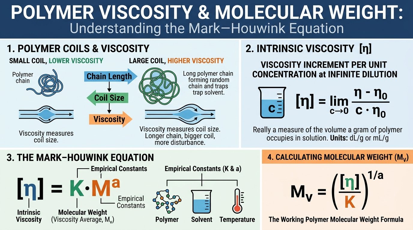
A dissolved polymer chain is not a compact particle. It is a random coil that sweeps out a volume thousands of times larger than the volume of its own atoms, trapping solvent inside and disturbing the flow of solvent around it. The longer the chain, the bigger the coil, the more it disturbs the flow, and the more viscous the solution becomes. That is the whole polymer molecular weight viscosity connection in one sentence: viscosity measures coil size, and coil size grows with chain length in a predictable way.
Two quantities make the idea exact. The intrinsic viscosity [η] is the viscosity increment a polymer produces per unit concentration in the limit of infinite dilution, when each coil acts alone; it has units of reciprocal concentration (dL/g or mL/g) and is really a measure of the volume a gram of polymer occupies in solution. The Mark–Houwink equation [η] = K·Ma then relates that volume to molecular weight through two empirical constants that depend on the polymer, the solvent and the temperature. Invert it and you have the working polymer molecular weight viscosity formula: Mv = ([η]/K)1/a. The molecular weights involved are the same kind of number our molecular weight calculator homepage computes for small molecules — grams per mole — but for a polymer they describe an average over a distribution of chain lengths.
Two things worth being clear about from the start. First, viscometry gives a particular average, the viscosity-average molecular weight Mv, which is weighted by Ma and therefore sits between the number average molecular weight Mn and the weight average molecular weight Mw, close to Mw. Second, the method is relative: K and a must first be calibrated against samples whose molecular weight is known absolutely (by light scattering, osmometry or mass spectrometry), which is why a polymer molecular weight viscosity table always states the solvent and temperature next to the constants. Use the wrong pair and the answer can be off by a factor of two.
How to Use This Calculator
The tool at the top of the page was built so that a polymer molecular weight viscosity question takes less time to solve than to read. Here is the workflow:
- Pick the mode that matches your data: an intrinsic viscosity or a molecular weight (Mode 1), flow times at several concentrations (Mode 2), a single flow-time pair (Mode 3), a melt viscosity (Mode 4), or a set of standards or fractions (Mode 5).
- Choose the polymer–solvent system from the library and K and a fill themselves in — or type your own constants. The library stores 25 systems from polystyrene in toluene to PET in phenol/tetrachloroethane, each with its temperature. K and [η] can be entered in dL/g or mL/g; the tool converts.
- Enter flow times as measured. Modes 2 and 3 take the solvent time t0 and the solution times in seconds (or ready-made relative viscosities), with concentrations in g/dL, g/mL, g/L or mg/mL.
- Press Calculate (or Enter). The headline result appears first, then the step-by-step derivation, a table of every derived quantity — ηrel, ηsp, reduced and inherent viscosities, intercepts, slopes, R² — and a bar chart such as the Huggins and Kraemer points converging on [η].
- Read the extras: Mode 1 reports the degree of polymerization, the Flory–Fox coil size and how much Mv would shift if a or K were slightly wrong; Mode 4 tells you the regime (above or below Mc) and the expected change in melt flow index.
- Export with Copy, CSV, TXT, Print or Share — and hit ↺ Reset before the next problem so stale inputs never contaminate a fresh calculation.
Your last ten results are stored in the history panel below the calculator (locally in your browser, nothing is uploaded). Clear All wipes it in one click. Click any preset chip to load a classic textbook example and see what a complete answer looks like.
The Five Modes Explained
📐 Mode 1 — Mark–Houwink: [η] ↔ Mv and Universal Calibration
The core polymer molecular weight viscosity conversion. Enter an intrinsic viscosity with K and a and the tool returns Mv = ([η]/K)1/a, the logarithmic form of the calculation, the degree of polymerization if you give the repeat-unit mass, and a sensitivity analysis showing how Mv moves when a changes by ±0.02 or K by ±10% — a sobering reminder that 1/a ≈ 1.45 amplifies every error in the constants. The Flory–Fox relation adds an estimate of the coil’s end-to-end distance, radius of gyration and hydrodynamic radius. The reverse option predicts [η] for a known M and tells you what specific viscosities to expect at typical concentrations. The third option performs universal GPC calibration: because a size-exclusion column separates by hydrodynamic volume [η]M, a polystyrene-equivalent molecular weight can be converted to the true M of your polymer from the two pairs of constants.
🧪 Mode 2 — Dilution Series with Huggins and Kraemer Fits
The proper laboratory route. Enter t0 and up to five (c, t) pairs and the tool computes ηrel, ηsp, ηsp/c and ln ηrel/c for every point, fits the Huggins line and the Kraemer line by least squares, reports both intercepts with kH, kK and R², averages them into [η] and checks that kH + kK is near 0.5. It warns when a point has ηrel above 2.0 (too concentrated for the linear equations) or below 1.1 (timing error dominates). With K and a supplied it finishes with Mv. Four polystyrene solutions in toluene with t0 = 100 s and t = 117.79, 137.55, 159.29 and 183.01 s at 0.2–0.8 g/dL give [η] = 0.840 dL/g, kH = 0.35 and Mv = 225,500 g/mol.
⚡ Mode 3 — Single-Point Intrinsic Viscosity
The quality-control shortcut. One concentration, two flow times. The tool brackets [η] between the inherent viscosity (lower bound) and the reduced viscosity (upper bound) and computes the Solomon–Ciuta estimate [η] = √(2(ηsp − ln ηrel))/c, the Deb–Chanda estimate, and — if you assume a Huggins constant — the Huggins solution. At c = 0.5 g/dL with t0 = 100 s and t = 148 s, ηrel = 1.48 and Solomon–Ciuta gives 0.839 dL/g, within 0.2% of the four-point value above.
🔥 Mode 4 — Melt Viscosity ↔ Mw
The other half of the polymer molecular weight viscosity story. Above the critical entanglement molecular weight the zero-shear melt viscosity of a linear polymer follows η0 = k·Mw3.4; below it, η0 is roughly proportional to Mw. Give one reference pair at the temperature of interest and the mode predicts η0 at a new Mw, or inverts a measured η0 to the Mw it implies, switching exponents at Mc if you supply it (typical values are listed: polyethylene 3,800, polystyrene 35,000, PMMA 27,500). Raising polystyrene from 200,000 to 300,000 g/mol multiplies η0 by 1.53.4 = 3.97 — 5,000 Pa·s becomes 19,850 Pa·s.
📊 Mode 5 — Fit K and a, or Average a Blend
Two calibration tasks. Enter the molecular weights and intrinsic viscosities of two to five narrow standards and a least-squares line through log [η] against log M returns a (the slope), K (from the intercept) and R², with the residual of every standard. Or enter the molecular weights and weights of up to five fractions and the mode returns Mn, Mw, Mz, the dispersity and the viscosity average Mv = (ΣwiMia)1/a, which is where you see directly that Mv lands about 90% of the way from Mn to Mw for a = 0.7 — the same machinery our polydispersity index calculator uses, extended to the viscosity average.
The Mark–Houwink Equation (With the Box You Should Memorize)
Every polymer molecular weight viscosity problem this page can pose — no exceptions — is one of these lines rearranged:
[η] = K·Mva ⇄ Mv = ([η] / K)1/a · log [η] = log K + a·log M
ηrel = t/t0 · ηsp = ηrel − 1 · [η] = limc→0 ηsp/c = limc→0 ln ηrel/c
Huggins: ηsp/c = [η] + kH[η]²c · Kraemer: ln ηrel/c = [η] − kK[η]²c · kH + kK ≈ 0.5 · η0 = k·Mw3.4 (M > Mc)
1 dL/g = 100 mL/g · a = 0.5 (θ solvent), 0.5–0.8 (good solvent), 1–2 (rod) · Mv = (ΣwiMia)1/a · Flory–Fox [η] = Φ⟨r²⟩3/2/M, Φ = 2.5×10²³ mol−1 · universal calibration: K1M11+a1 = K2M21+a2
Two details in that polymer molecular weight viscosity box decide most marks. First, K and [η] must be in the same unit. Handbooks quote K in dL/g (typical values 10−4–10−3) or in mL/g (100 times larger); mixing them multiplies Mv by 1001/a, roughly a factor of 800 for a = 0.7. Second, the constants belong to a system, not a polymer. Polystyrene in toluene at 25 °C (K = 1.7 × 10⁻⁴, a = 0.69) and polystyrene in cyclohexane at 34.5 °C (K = 8.2 × 10⁻⁴, a = 0.50) are different calibrations of the same molecule, because the coil is swollen in the first solvent and unperturbed in the second.
Notice also what the formula rewards: logarithms. Because the exponent is fractional, the cleanest way to solve any polymer molecular weight viscosity problem by hand is log M = (log [η] − log K)/a. For [η] = 0.84 dL/g: log 0.84 = −0.0757, log (1.7 × 10⁻⁴) = −3.7696, so log M = 3.6939/0.69 = 5.3534 and Mv = 225,600 g/mol. Three lines, no fractional powers on the calculator, and an answer you can check against a plot.
Relative, Specific, Reduced, Inherent and Intrinsic Viscosity
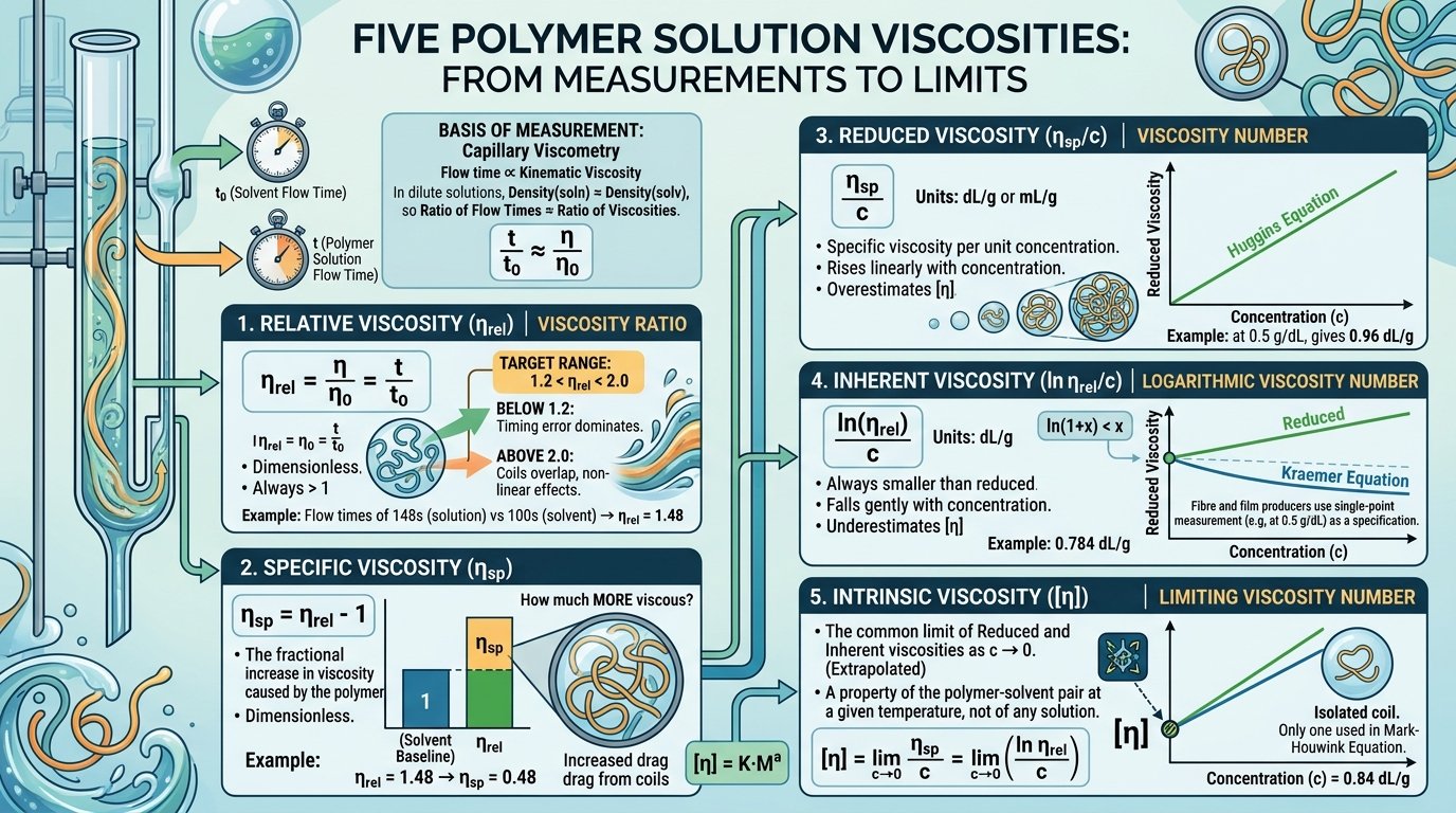
Five names for four ratios and one limit trip up more students than the Mark–Houwink equation itself, yet they are the vocabulary of every polymer molecular weight viscosity problem. In a capillary viscometer the flow time is proportional to the kinematic viscosity, and because dilute polymer solutions have practically the solvent’s density, the ratio of flow times is the ratio of viscosities.
Relative viscosity, ηrel = η/η0 = t/t0
Dimensionless and always greater than 1. IUPAC’s name is the viscosity ratio. Good practice keeps it between about 1.2 and 2.0: below 1.2 the difference between the two times is a few seconds and timing error dominates; above 2.0 the coils overlap and the Huggins and Kraemer equations stop being linear.
Specific viscosity, ηsp = ηrel − 1
The fractional increase in viscosity caused by the polymer. Also dimensionless. For a solution flowing in 148 s against a solvent time of 100 s, ηrel = 1.48 and ηsp = 0.48.
Reduced viscosity, ηsp/c (the viscosity number)
Specific viscosity per unit concentration, in dL/g or mL/g. It rises linearly with concentration in dilute solution because coils begin to interact — that is the Huggins equation — so at any finite concentration it over-estimates [η]. At 0.5 g/dL the example above gives 0.96 dL/g.
Inherent viscosity, ln ηrel/c (the logarithmic viscosity number)
Because ln(1 + x) < x, the inherent viscosity is always smaller than the reduced viscosity and it under-estimates [η], falling gently with concentration: the Kraemer equation. The same solution gives ln 1.48/0.5 = 0.784 dL/g. Fibre and film producers often quote the inherent viscosity at a standard concentration (0.5 g/dL is common for PET and nylon) as a specification in its own right.
Intrinsic viscosity, [η] (the limiting viscosity number)
The common limit of the reduced and inherent viscosities as c → 0, when each coil is alone in the solvent. It is a property of the polymer–solvent pair at that temperature, not of any solution, and it is the only one of the five that goes into the Mark–Houwink equation. In the example the two bounds are 0.784 and 0.96 dL/g and the extrapolated value is 0.84. Note that every polymer molecular weight viscosity handbook uses square brackets for it — [η] — and that its unit is the inverse of a concentration, which is why K carries the same unit.
What K and a Really Mean: Solvent Quality, the θ Condition and Chain Shape
The Mark–Houwink constants look like fudge factors but they encode real physics, and reading them correctly is what separates a polymer molecular weight viscosity answer from a polymer molecular weight viscosity explanation.
The exponent a reports the shape of the dissolved chain. Einstein showed in 1906 that rigid spheres raise viscosity by a fixed 2.5 times their volume fraction regardless of size, so a compact sphere has a = 0. A flexible chain in a θ solvent — the temperature at which polymer–solvent and polymer–polymer contacts are equally favourable and the coil takes its unperturbed random-walk dimensions — has a = 0.5, exactly. In a good solvent the coil swells to avoid its own segments, its size grows faster than M1/2, and a rises to 0.6–0.8, the Flory limit for a fully swollen coil being 0.8. Stiff chains — cellulose derivatives, aromatic polyamides — give 0.8–1.0, and rigid rods such as DNA, xanthan or poly(γ-benzyl glutamate) give 1.0–1.8. So a = 0.69 for polystyrene in toluene says: flexible coil, moderately good solvent.
The prefactor K sets the scale. It is larger in poor solvents (compare 8.2 × 10⁻⁴ in cyclohexane with 1.7 × 10⁻⁴ in toluene) because a smaller exponent must be compensated to reproduce the same [η] at the calibration molecular weights, and it falls as a rises. K and a are therefore strongly correlated: quoting one without the other, or mixing a K from one paper with an a from another, is meaningless. In a θ solvent K has a special interpretation, Kθ = Φ(⟨r²⟩0/M)3/2, which links viscometry to the unperturbed dimensions of the chain.
The Flory–Fox relation makes the polymer molecular weight viscosity link a statement about size. [η] = Φ⟨r²⟩3/2/M with Φ ≈ 2.5 × 10²³ mol−1 (for [η] in mL/g and r in cm) says that intrinsic viscosity is coil volume per unit mass. For the polystyrene example — [η] = 84 mL/g, Mv = 225,600 — the root-mean-square end-to-end distance comes out at about 42 nm and the radius of gyration at about 17 nm: a molecule 2 nm thick spread over a sphere 35 nm across, 95% of which is solvent. That is why a fraction of a percent of polymer can double the viscosity of a liquid.
Temperature and solvent shift both constants. Warming a good solvent usually lowers a slightly (the coil is already swollen); warming a poor solvent through the θ temperature raises a from 0.5 upward. This is the reason the polymer molecular weight viscosity literature attaches a temperature to every K–a pair, and the reason an Ubbelohde bath is thermostatted to ±0.02 °C: a 1 °C drift changes flow times by about 2% and, through 1/a, molecular weight by about 3%. Rigid molecules are the extreme case; for them the same reasoning explains why the Mark–Houwink exponent of DNA depends on ionic strength, which stiffens or relaxes the double helix.
Three Worked Examples, Step by Step
Example 1 — The classic polymer molecular weight viscosity problem: [η] to Mv
Problem: A polystyrene sample has an intrinsic viscosity of 0.84 dL/g in toluene at 25 °C. With K = 1.7 × 10⁻⁴ dL/g and a = 0.69, find the viscosity-average molecular weight and the degree of polymerization.
Step 1 — Units: [η] and K are both in dL/g. Good. (If the handbook had given K = 1.7 × 10⁻² mL/g, we would convert [η] to 84 mL/g first.)
Step 2 — Logarithms: log M = (log 0.84 − log 1.7 × 10⁻⁴)/0.69 = (−0.0757 + 3.7696)/0.69 = 5.3534.
Step 3 — Molecular weight: Mv = 105.3534 = 225,600 g/mol. Degree of polymerization = 225,600 / 104.15 (styrene) = 2,166 repeat units.
Check: K·Ma = 1.7 × 10−4 × 225,6000.69 = 0.84 dL/g. Sensitivity: had a been 0.71 the answer would be 159,000, had it been 0.67, 326,000 — a ±0.02 uncertainty in a is a factor of two in M. Quote the constants with the result.
Example 2 — A dilution series with Huggins and Kraemer extrapolation
Problem: Toluene flows through an Ubbelohde viscometer in 100.00 s at 25 °C. Polystyrene solutions of 0.2, 0.4, 0.6 and 0.8 g/dL flow in 117.79, 137.55, 159.29 and 183.01 s. Find [η], the Huggins constant and Mv.
Step 1 — Ratios: ηrel = 1.1779, 1.3755, 1.5929, 1.8301; ηsp = 0.1779, 0.3755, 0.5929, 0.8301.
Step 2 — Reduced and inherent: ηsp/c = 0.8895, 0.9388, 0.9882, 1.0376 dL/g; ln ηrel/c = 0.8187, 0.7970, 0.7759, 0.7555 dL/g. One rises, one falls — as they should.
Step 3 — Fits: Huggins line: intercept 0.8401, slope 0.2469 → kH = 0.2469/0.8401² = 0.35. Kraemer line: intercept 0.8395, slope −0.1054 → kK = 0.15. kH + kK = 0.50 — the two plots are consistent.
Step 4 — Result: [η] = (0.8401 + 0.8395)/2 = 0.840 dL/g; Mv = (0.840/1.7 × 10−4)1/0.69 = 225,500 g/mol. A Huggins constant of 0.35 is typical of a good solvent; 0.5–0.7 would suggest a θ solvent and anything above 0.8 aggregation.
Example 3 — Melt viscosity: what a 50% higher Mw does to processing
Problem: A polystyrene grade with Mw = 200,000 g/mol has a zero-shear melt viscosity of 5,000 Pa·s at 200 °C. Estimate the viscosity of a grade with Mw = 300,000 at the same temperature, and the Mw of a grade that measures 1,250 Pa·s.
Step 1 — Regime: both grades are far above Mc for polystyrene (about 35,000), so η0 ∝ Mw3.4 applies.
Step 2 — Ratio: (300,000/200,000)3.4 = 1.53.4 = 3.97; η0 = 5,000 × 3.97 = 19,850 Pa·s.
Step 3 — Inverse: 1,250/5,000 = 0.25; Mw = 200,000 × 0.251/3.4 = 133,000 g/mol.
Meaning: A 50% increase in chain length quadruples the melt viscosity; a 33% decrease quarters it. Melt flow index runs roughly inversely, so the 300,000 grade would flow about a quarter as fast through the standard die. This is the polymer molecular weight viscosity trade-off every resin producer manages: higher Mw for toughness and melt strength, lower Mw for processability.
Reference Table: Mark–Houwink Constants for Common Polymers
Keep this table beside you when checking a polymer molecular weight viscosity answer. The values are typical literature figures of the kind tabulated in the Polymer Handbook; published constants for the same system vary by 10–30% between sources and molecular-weight ranges, so for a certificate of analysis use the pair specified by your standard or measured on your own calibrants. K is in dL/g; multiply by 100 for mL/g.
| Polymer | Solvent | T (°C) | K (dL/g) | a | Note |
|---|---|---|---|---|---|
| Polystyrene | toluene | 25 | 1.7 × 10⁻⁴ | 0.69 | good solvent, the textbook system |
| Polystyrene | THF | 25 | 1.41 × 10⁻⁴ | 0.70 | GPC eluent; universal-calibration reference |
| Polystyrene | cyclohexane | 34.5 | 8.2 × 10⁻⁴ | 0.50 | θ solvent — unperturbed coil |
| Poly(methyl methacrylate) | acetone | 25 | 7.5 × 10⁻⁵ | 0.70 | good solvent |
| Poly(methyl methacrylate) | THF | 25 | 1.04 × 10⁻⁴ | 0.697 | GPC eluent |
| Polyethylene (linear) | decalin | 135 | 6.2 × 10⁻⁴ | 0.70 | ASTM D1601 conditions |
| Polyethylene (linear) | 1,2,4-trichlorobenzene | 135 | 7.36 × 10⁻⁴ | 0.67 | high-temperature GPC eluent |
| Polypropylene (isotactic) | decalin | 135 | 1.10 × 10⁻⁴ | 0.80 | near the good-solvent limit |
| Poly(vinyl chloride) | THF | 25 | 1.63 × 10⁻⁴ | 0.766 | industry also uses the Fikentscher K-value |
| Polyisobutylene | benzene | 24 | 1.07 × 10⁻³ | 0.50 | θ solvent |
| cis-1,4-Polybutadiene | cyclohexane | 25 | 3.43 × 10⁻⁴ | 0.70 | synthetic rubber |
| Natural rubber (cis-polyisoprene) | toluene | 25 | 5.02 × 10⁻⁴ | 0.667 | Mooney viscosity used in the trade |
| Polydimethylsiloxane | toluene | 25 | 2.0 × 10⁻⁴ | 0.66 | silicone fluids |
| Polycarbonate | THF | 25 | 4.4 × 10⁻⁴ | 0.69 | engineering plastic |
| Poly(ethylene terephthalate) | phenol/TCE 60:40 | 25 | 7.44 × 10⁻⁴ | 0.648 | “IV” of bottle and fibre grades |
| Poly(ethylene oxide) | water | 25 | 1.25 × 10⁻⁴ | 0.78 | water-soluble, highly expanded |
| Polyacrylonitrile | DMF | 30 | 3.01 × 10⁻⁴ | 0.75 | acrylic fibre precursor |
Three polymer molecular weight viscosity patterns worth noticing. Every θ-solvent entry has a = 0.50 and a K several times larger than the good-solvent entry for the same polymer — the two constants move in opposite directions. The industrial polyolefins are measured at 135 °C because they do not dissolve below about 100 °C, which is also why their GPC is run hot. And for the same polymer in two good solvents (polystyrene in toluene and THF) the constants agree within 20%, so a rough answer is possible with a neighbouring system, but a certificate is not.
Measuring It in the Lab: Ubbelohde, Ostwald, Melt Rheometer and GPC-Viscometry
Four instruments produce almost every polymer molecular weight viscosity number in the literature, and each has a niche in the polymer molecular weight viscosity workflow.
The Ubbelohde suspended-level viscometer — the standard for [η]. A glass U-tube with a bulb above a fine capillary; the liquid is drawn up, released, and the time for the meniscus to pass two marks is recorded. Leo Ubbelohde’s design of the 1930s adds a third arm that vents the bottom of the capillary, so the flow time does not depend on how much liquid is in the reservoir — which means the solution can be diluted in situ, four or five concentrations from one filling. Flow times of 100–200 s for the solvent keep the kinetic-energy correction below 0.5%; the bath is held to ±0.02 °C; and the solutions are filtered because a single dust fibre in a 0.5 mm capillary ruins a run. ISO 1628 and ASTM D2857 codify the procedure.
The Ostwald viscometer — the teaching instrument. Simpler, cheaper, and the one most students meet in their first polymer molecular weight viscosity practical. Because the driving head depends on the volume charged, exactly the same volume must be pipetted for every solution, so dilution in the viscometer is not possible. Accuracy is fine for a laboratory course and for the reduced-viscosity specifications of the older standards.
The rotational or capillary melt rheometer — for η0. A parallel-plate or cone-and-plate rheometer sheared slowly enough to reach the Newtonian plateau gives the zero-shear viscosity that the 3.4-power law needs; a capillary rheometer gives the shear-thinning curve used for process design; and the melt-flow indexer (ASTM D1238), a dead-weight capillary extruder, gives the single-point melt flow index that resin datasheets quote. All three read chain length through entanglement rather than through coil volume, which is why they track Mw rather than Mv.
GPC with an on-line viscometer — the modern absolute route. A differential viscometer after the size-exclusion columns measures [η] slice by slice as the polymer elutes. Combined with the concentration detector and a universal calibration curve it returns the whole molecular-weight distribution, the Mark–Houwink plot of the sample itself (a straight line whose slope is a), and — from deviations of that line — the amount of long-chain branching. It is the method that measures the K and a values the rest of us look up.
Whatever the instrument, the polymer molecular weight viscosity reduction is identical: flow times to ηrel and ηsp, extrapolation to [η], Mark–Houwink to Mv. The absolute methods that calibrate it have their own pages: the colligative routes to Mn through osmotic pressure, freezing point depression and boiling point elevation, and the mass-spectrometric routes through the exact mass calculator and monoisotopic mass calculator for oligomers small enough to fly.
Who Uses the Polymer Molecular Weight Viscosity Relationship?
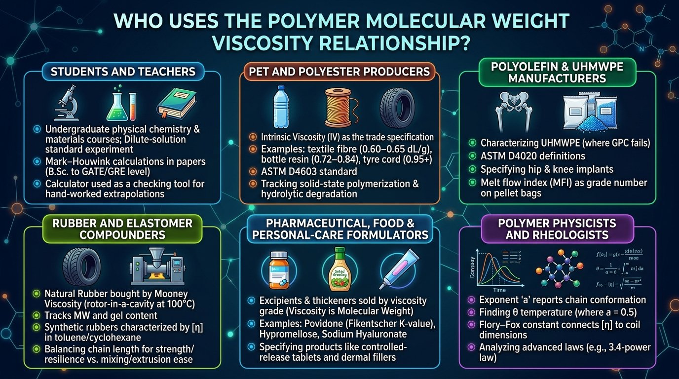
Students and teachers. Dilute-solution viscometry is the standard polymer-characterization experiment in every undergraduate physical chemistry and materials course, and Mark–Houwink calculations appear in polymer chemistry papers from B.Sc. to GATE and GRE subject level. A polymer molecular weight viscosity calculator that shows every step is a checking tool, not a shortcut: work the extrapolation by hand, then compare.
PET and polyester producers. The intrinsic viscosity (“IV”) of poly(ethylene terephthalate) is the polymer molecular weight viscosity specification of the trade: 0.60–0.65 dL/g for textile fibre, 0.72–0.84 for bottle resin, 0.95 and above for tyre cord, all measured by ASTM D4603 in phenol/tetrachloroethane. With the constants in the table, an IV of 0.80 corresponds to Mv of roughly 48,000 g/mol; solid-state polymerization exists to push IV up, and hydrolytic degradation during moulding shows up first as IV loss.
Polyolefin and UHMWPE manufacturers. Ultra-high-molecular-weight polyethylene cannot be characterized by GPC (it barely dissolves and shears in the columns), so ASTM D4020 defines it by dilute-solution viscosity in decalin at 135 °C; an intrinsic viscosity of 20 dL/g corresponds to Mv of about 3.2 million g/mol, and the hip and knee implants made from it are specified that way. For ordinary polyethylene and polypropylene the melt flow index — the other end of the polymer molecular weight viscosity spectrum — is the grade number printed on every bag of pellets.
Rubber and elastomer compounders. Natural rubber is bought by Mooney viscosity, a polymer molecular weight viscosity index of its own, a rotor-in-a-cavity measurement at 100 °C that tracks molecular weight and gel content; synthetic rubbers are also characterized by [η] in toluene or cyclohexane. Both feed the same decision: enough chain length for strength and resilience, little enough for mixing and extrusion.
Pharmaceutical, food and personal-care formulators. Excipients and thickeners are sold by viscosity grade because viscosity is molecular weight: povidone by Fikentscher K-value (K-30 around 50,000 g/mol, K-90 above a million), hypromellose by the viscosity of a 2% solution, sodium hyaluronate, carbomers, xanthan, guar and carboxymethylcellulose likewise. A dermal filler, a controlled-release tablet matrix and a salad dressing are all specified through the polymer molecular weight viscosity link.
Polymer physicists and rheologists. The exponent a reports chain conformation, the θ temperature is found where a = 0.5, the Flory–Fox constant connects [η] to coil dimensions measured by light scattering, and the 3.4-power law was the experimental fact that reptation theory had to explain. Blends of different molecular weights — whose averages the average molecular weight of a mixture tool handles for small molecules and Mode 5 handles for polymer fractions — are the standard way of tuning melt viscosity without changing the polymer.
Full Lab Walkthrough: Mv of a Polystyrene Sample
Suppose you are handed an unknown polystyrene, a bottle of toluene, an Ubbelohde viscometer, a 25 °C water bath and a 10 mL pipette. Here is the complete polymer molecular weight viscosity workflow, with the numbers a good run produces.
- Make the stock solution. Weigh 0.2000 g of polymer into a 25 mL volumetric flask, add toluene, and leave it overnight with occasional swirling — high polymers dissolve slowly and shaking can shear long chains. Make up to the mark at 25 °C: 0.800 g/dL.
- Filter everything. Pass the solvent and the stock through a 0.45 µm PTFE syringe filter straight into the viscometer. Dust is the number-one cause of scattered flow times.
- Time the solvent. Charge 10.00 mL of toluene, equilibrate 10 minutes in the bath, draw the liquid above the upper mark, release and time the meniscus between the marks. Repeat until three readings agree within 0.2 s: t0 = 100.00 s.
- Time the stock. Empty, rinse with stock, charge 10.00 mL of stock, equilibrate and time: 183.01 s. ηrel = 1.830, inside the 1.2–2.0 window — good.
- Dilute in the viscometer. Add 2.50, then 3.33, then 10.00 mL of filtered toluene (each addition mixed by bubbling filtered air for a minute and re-equilibrated) to give 0.6, 0.4 and 0.2 g/dL, timing each: 159.29, 137.55 and 117.79 s. Concentrations are corrected for the actual volumes if the pipette deliveries differ.
- Reduce the data. For each point compute ηrel, ηsp, ηsp/c and ln ηrel/c: reduced viscosities 0.8895, 0.9388, 0.9882 and 1.0376 dL/g; inherent viscosities 0.8187, 0.7970, 0.7759 and 0.7555 dL/g.
- Plot and extrapolate. Both lines against c on one graph: Huggins intercept 0.8401 dL/g (kH = 0.35), Kraemer intercept 0.8395 dL/g (kK = 0.15); they meet within 0.1%, and kH + kK = 0.50. [η] = 0.840 dL/g. Mode 2 with the five times reproduces every number.
- Convert and report. With K = 1.7 × 10⁻⁴ dL/g and a = 0.69 (polystyrene/toluene/25 °C), Mv = (0.840/1.7 × 10−4)1/0.69 = 225,500 g/mol. Report it as “Mv = 2.26 × 10⁵ g/mol, toluene, 25 °C, K = 1.7 × 10⁻⁴ dL/g, a = 0.69″, because without the constants the number cannot be reproduced.
Two lessons from the walkthrough. The Huggins and Kraemer intercepts agreeing to 0.1% is the internal quality check — if they differ by several percent, a concentration is wrong or a point is too concentrated. And the polymer molecular weight viscosity result is only as good as the constants: with the THF pair (1.41 × 10⁻⁴, 0.70) the same [η] would read 249,000, a 10% difference from the solvent alone, which is why the report names the system.
A Short History: Staudinger, Mark, Houwink and Flory
The polymer molecular weight viscosity connection was the first evidence that macromolecules exist. In the 1920s most chemists believed rubber, cellulose and starch were colloidal aggregates of small molecules held together by weak forces. Hermann Staudinger insisted they were covalent chains thousands of atoms long, and his strongest argument was that their solutions were far too viscous for small molecules and stayed viscous whatever the solvent. In 1930 he proposed the first quantitative polymer molecular weight viscosity law, ηsp/c = Km·M, with the specific viscosity proportional to molecular weight because he pictured the chains as rigid rods. The law was wrong in detail but right in spirit, and it earned him the 1953 Nobel Prize.
The correction to Staudinger’s polymer molecular weight viscosity law came from thinking about shape. Werner Kuhn showed in 1934 that a flexible chain coils up, and that a coil’s contribution to viscosity should grow more slowly than its length. Herman Mark in 1938 and Roelof Houwink in 1940 (with Ichiro Sakurada independently in Japan the same year) wrote the empirical relation [η] = K·Ma with an exponent between 0.5 and 1, and it has carried their names ever since — Mark–Houwink, Mark–Houwink–Sakurada, or KMHS with Kuhn included. The concentration-dependence equations followed quickly: Elmer Kraemer’s logarithmic form in 1938 and Maurice Huggins’s linear form in 1942, the pair every dilution series still uses.
Paul Flory turned the empirical constants into physics. His 1949 theory of the excluded-volume coil explained why a rises above 0.5 in a good solvent, his θ-temperature concept identified where it equals 0.5 exactly, and the 1951 Flory–Fox equation [η] = Φ⟨r²⟩3/2/M tied the intrinsic viscosity to the coil’s dimensions. In 1948 Fox and Flory also reported that the melt viscosity of polystyrene rose as M3.4 above a critical chain length — an exponent so universal that Pierre-Gilles de Gennes’s 1971 reptation model (which predicts 3.0) and the Doi–Edwards theory of 1978 were judged partly by how close they came to it. Flory received the Nobel Prize in 1974, de Gennes in 1991.
The last chapter belongs to instruments. Benoit, Grubisic and Rempp showed in 1967 that a gel-permeation column separates by hydrodynamic volume [η]M, giving the universal calibration that Mode 1 performs; on-line viscometers in the 1980s made [η] a routine output of every GPC run; and today a triple-detector chromatograph measures K and a for a new polymer in an afternoon. The mass spectrometer, which weighs single molecules to a millionth of a unit (see our isotopic mass calculator and the comparison of average vs monoisotopic mass), has taken over below a few thousand daltons — but for the million-dalton chains in a tyre or a hip joint, Staudinger’s capillary is still the instrument of record.
Melt Viscosity and the 3.4-Power Law in Industry
Solution viscometry measures chain length gently; the melt end of the polymer molecular weight viscosity spectrum measures it brutally. Below a critical molecular weight Mc the chains slide past one another and η0 grows roughly in proportion to Mw. Above Mc — about 3,800 g/mol for polyethylene, 27,500 for PMMA, 35,000 for polystyrene — each chain is threaded through a mesh of its neighbours and can move only by snaking along its own contour, and η0 jumps to the 3.4 power. The consequences run through every polymer factory.
Grade design. Doubling Mw multiplies zero-shear viscosity by 23.4 = 10.6; a 10% increase costs 38% in viscosity. Toughness, environmental stress-crack resistance and melt strength all improve with Mw, so producers push chain length up to the point where the extruder or injection machine cannot cope, then broaden the distribution or add a low-Mw tail as an internal lubricant. Because the law is weighted toward Mw (strictly, a slightly higher average), the long chains in a broad distribution dominate: two resins with the same Mn can differ several-fold in melt viscosity.
Melt flow index as a molecular-weight proxy. The MFI test extrudes the melt through a standard die under a standard weight and reports grams per 10 minutes; it is roughly inversely proportional to η0, so it falls as Mw−3.4. An MFI of 2 versus 20 g/10 min for the same polyethylene family therefore implies a molecular-weight ratio of only about 101/3.4 = 2, which is why small MFI differences correspond to real grade differences. Mode 4 converts either way, and a polymer molecular weight viscosity calculation of this kind is the fastest sanity check on a datasheet.
Degradation and recycling. The polymer molecular weight viscosity link also works as an alarm: chain scission during processing — hydrolysis of PET and nylon by traces of moisture, oxidation of polyolefins, shear of UHMWPE — lowers Mw, and the 3.4 exponent makes viscosity an exquisitely sensitive detector: a 5% loss of Mw is a 16% loss of melt viscosity. Recyclers track IV of PET flake and MFI of polyolefin regrind for exactly this reason, and chain extenders exist to reverse it.
Branching and additives. Long-chain branching raises η0 above the linear 3.4-law prediction at the same Mw while making the melt more shear-thinning; short-chain branching barely matters; plasticizers lower viscosity by lowering the glass transition rather than the chain length. The power law applies to linear chains at one temperature; change the temperature and the whole curve shifts by the Arrhenius or WLF factor, which is why Mode 4 asks for a reference pair at the temperature you care about.
Practice Problems (With Answers)
Work each problem by hand first, then verify with the free polymer molecular weight viscosity calculator above. Answers are hidden until you click.
Problem 1 — Predict the intrinsic viscosity of PMMA with M = 200,000 g/mol in acetone at 25 °C (K = 7.5 × 10⁻⁵ dL/g, a = 0.70).
log [η] = log 7.5 × 10⁻⁵ + 0.70 × log 200,000 = −4.1249 + 0.70 × 5.3010 = −0.4142, so [η] = 0.385 dL/g = 38.5 mL/g. A 0.5 g/dL solution would show ηsp ≈ 0.385 × 0.5 + 0.35 × 0.385² × 0.25 = 0.21, i.e. a flow time about 21% longer than acetone — a sensible working concentration.
Problem 2 — Linear polyethylene has [η] = 1.50 dL/g in decalin at 135 °C (K = 6.2 × 10⁻⁴ dL/g, a = 0.70). Find Mv and the degree of polymerization.
Mv = (1.50/6.2 × 10−4)1/0.70 = 2,4191.4286 = 68,200 g/mol. Degree of polymerization = 68,200/28.05 (ethylene) = 2,430 — about 4,860 backbone carbons, a chain roughly 0.6 µm long if stretched out, coiled into a sphere some 20 nm across.
Problem 3 — A single 0.5 g/dL polystyrene solution flows in 148.0 s against 100.0 s for toluene. Estimate [η] by the Solomon–Ciuta method and Mv (K = 1.7 × 10⁻⁴, a = 0.69).
ηrel = 1.480, ηsp = 0.480, ln ηrel = 0.3920. [η] = √(2(0.480 − 0.3920))/0.5 = √0.1759/0.5 = 0.4194/0.5 = 0.839 dL/g, bracketed by the inherent viscosity 0.784 and the reduced viscosity 0.960. Mv = (0.839/1.7 × 10−4)1/0.69 = 225,000 g/mol, within 0.2% of the four-point result in Example 2.
Problem 4 — Two narrow polystyrene standards give [η] = 0.1578 dL/g at M = 20,000 and 1.247 dL/g at M = 400,000 in toluene. Find K and a.
a = log(1.247/0.1578)/log(400,000/20,000) = log 7.902/log 20 = 0.8977/1.3010 = 0.690. K = 0.1578/20,0000.690 = 0.1578/928.6 = 1.70 × 10⁻⁴ dL/g. Two points fix a line but give no R²; Mode 5 with four standards (adding 50,000/0.297 and 100,000/0.4791) returns the same constants with R² = 1.000.
Problem 5 — Equal weights of two monodisperse fractions, M = 50,000 and 500,000, are blended. Find Mn, Mw, Mv (a = 0.70) and the dispersity, and say which average viscometry would report.
wi = 0.5 each. Mn = 1/(0.5/50,000 + 0.5/500,000) = 90,900; Mw = 0.5 × 50,000 + 0.5 × 500,000 = 275,000; Mv = (0.5 × 50,0000.7 + 0.5 × 500,0000.7)1/0.7 = 240,900; Đ = 275,000/90,900 = 3.03. Viscometry reports Mv, 88% of Mw and 2.65 times Mn — so comparing a Mark–Houwink result with an osmometric Mn for this blend would look like a 165% “error” when both are correct.
Tips for Fast, Error-Free Calculations
- ✅ Match the units of K and [η] before anything else — the number-one polymer molecular weight viscosity habit. dL/g and mL/g differ by 100, and the mismatch is raised to the power 1/a, so it does not produce a small error but a ridiculous one (a factor of several hundred). Write the unit next to K on the page.
- ✅ Solve in logarithms. log M = (log [η] − log K)/a is three calculator keystrokes for any polymer molecular weight viscosity problem and avoids fractional powers of tiny numbers; it is also the form you plot to find K and a from standards.
- ✅ Keep ηrel between 1.2 and 2.0. Choose concentrations so that the most dilute solution still flows at least 20% slower than the solvent and the most concentrated no more than twice as slowly; outside that window the Huggins and Kraemer lines curve.
- ✅ Use both extrapolations and check kH + kK ≈ 0.5. Two intercepts that agree are your evidence that the data are good; kH alone tells you the solvent quality (0.3–0.4 good, 0.5–0.7 θ).
- ✅ Report Mv as Mv, with the constants. A polymer molecular weight viscosity result is a viscosity average. Compare it with Mw from GPC or light scattering, not with Mn from osmometry or end-group analysis; and always state solvent, temperature, K and a so the number can be reproduced.
- ✅ Reset between problems — the ↺ Reset button on each mode of the polymer molecular weight viscosity calculator keeps an old K, a or t0 from contaminating the next calculation, which is the most common cause of a “the tool is wrong” moment.
⚗️ Pro workflow: Mode 2 to reduce a dilution series to [η] with both extrapolations → Mode 1 to convert it to Mv with the library constants and read the sensitivity → Mode 3 for the daily QC single-point check once the Huggins constant of your system is known → Mode 5 to calibrate your own K and a when the literature pair does not fit your grade → Mode 4 when the question moves from the flask to the extruder. Export the steps with Copy or Print and paste them straight into the report.
5 Common Mistakes to Avoid
A decade of marking polymer molecular weight viscosity answers produces the same five errors on repeat:
- Using ηsp/c at a single concentration as if it were [η]. The reduced viscosity over-estimates the intrinsic viscosity by kH[η]²c — 14% in Example 2 at 0.5 g/dL — and the error is raised to 1/a in Mv. Extrapolate, or at least use a single-point formula.
- Taking polymer molecular weight viscosity constants for the wrong solvent or temperature. Polystyrene constants in cyclohexane at 34.5 °C applied to a toluene measurement give a molecular weight that is wrong by a factor of two or more. The K–a pair belongs to a system; the library in Mode 1 names the system for this reason.
- Mixing K in mL/g with [η] in dL/g. A K of 1.7 × 10⁻² is the toluene constant in mL/g, not a different measurement. If your Mv comes out in the billions or the hundreds, this is why.
- Comparing Mv with Mn and calling the difference an error. For a typical polydisperse sample Mv is 1.7–1.9 times Mn and 0.85–0.95 of Mw; both numbers are right, they are different averages. Osmometry and viscometry on the same sample are supposed to disagree.
- Applying the 3.4-power law below Mc, to branched polymers, or across temperatures. Below the entanglement threshold the exponent is about 1; long-chain branching raises the viscosity above the linear prediction; and comparing a 190 °C melt with a 230 °C melt needs a temperature shift factor first. Mode 4 asks for Mc and a reference pair at one temperature for exactly these reasons.
How This Calculator Is Different
| Feature | This calculator | Generic Mark–Houwink tool | By hand |
|---|---|---|---|
| K and a library (25 polymer–solvent–temperature systems) | ✅ One click, unit conversion dL/g ↔ mL/g | ⚠️ Usually you type K and a | Handbook lookup |
| Sensitivity of Mv to K and a, Flory–Fox coil size, DP | ✅ Reported with every result | ❌ | Rarely done |
| Dilution series: Huggins + Kraemer least squares, kH, kK, R², range warnings | ✅ Up to 5 points, flow times or ηrel, 4 concentration units | ❌ | Graph paper or spreadsheet |
| Single-point [η]: Solomon–Ciuta, Deb–Chanda, Huggins with bounds | ✅ All three, bracketed | ❌ | ✅ Slow |
| Melt viscosity ↔ Mw with Mc switch and custom exponent | ✅ Both directions, regime named, MFI hint | ❌ | ✅ |
| Universal GPC calibration, K & a fitting, blend averages (Mn, Mw, Mv, Mz) | ✅ With residuals and R² | ❌ | Spreadsheet |
| Export & history | ✅ CSV/TXT/print/share + last 10 | ❌ Usually none | Notebook |
Related polymer molecular weight viscosity companions carry the theme onward. The three polymer averages have their own pages — number average, weight average and the polydispersity index that relates them. The repeat-unit masses that turn Mv into a degree of polymerization come from the atomic mass calculator and the formula weight calculator; converting a weighed sample to moles of chains is a job for the grams to moles calculator, and solution concentrations in mol/L for the molarity calculator. For the small-molecule routes to molar mass that calibrate polymer methods, see molecular weight from vapor density and molar mass from gas density; for reactive-group bookkeeping in resins and hardeners, the equivalent weight calculator; and for reaction stoichiometry and hydrated reagents, the stoichiometry calculator and molar mass of hydrates calculator.
Where the Numbers Come From
The Mark–Houwink constants in this polymer molecular weight viscosity calculator are typical literature values of the kind compiled in the Polymer Handbook (Brandrup, Immergut and Grulke) and the polymer-physics literature; each entry carries its solvent and temperature, and the values are given in dL/g with automatic conversion to mL/g. Published constants for one system differ between laboratories and molecular-weight ranges by 10–30%, and because Mv depends on them through the power 1/a, that spread is inherited — which is why every result also shows how Mv shifts for a ± 0.02 and K ± 10%. The Flory–Fox constant is taken as Φ = 2.5 × 10²³ mol−1 with [η] in mL/g; the melt exponent defaults to 3.4 with typical critical entanglement molecular weights from rheological compilations; the Solomon–Ciuta and Deb–Chanda formulas are the original 1962 and 1966 forms. Repeat-unit masses use IUPAC 2021 atomic weights (styrene 104.15, ethylene 28.05, methyl methacrylate 100.12, ethylene terephthalate 192.17 g/mol).
Standards referenced in the text: ISO 1628 and ASTM D2857 (dilute-solution viscosity of polymers), ASTM D4603 (PET intrinsic viscosity), ASTM D1601 (polyethylene), ASTM D4020 (UHMWPE), ASTM D1238 (melt flow rate). If you spot a discrepancy worth checking, our corrections policy explains how reports are handled, and the contact page is the fastest way to reach us; more about the site and its author is on the about page.
Exam Checklist
☐ I can write the Huggins and Kraemer equations, explain why one rises and one falls with c, and extrapolate both to the common intercept [η].
☐ I can state the Mark–Houwink polymer molecular weight viscosity equation, solve it in logarithms for Mv, and explain why K and a belong to a polymer–solvent–temperature system.
☐ I know that a = 0.5 in a θ solvent, 0.5–0.8 for flexible coils in good solvents and 1–2 for rods, and what each says about chain shape.
☐ I can place Mv between Mn and Mw, compute it for a blend from (ΣwiMia)1/a, and say which absolute method it should be compared with.
☐ I can use a single-point formula (Solomon–Ciuta) and state when it is and is not adequate.
☐ I can apply η0 ∝ Mw3.4 above Mc, know typical Mc values, and explain the exponent through entanglement and reptation.
☐ I’ve verified my practice answers with the polymer molecular weight viscosity calculator above.
Frequently Asked Questions
How is polymer molecular weight related to viscosity?
In dilute solution through the Mark–Houwink equation [η] = K·Ma: the intrinsic viscosity grows as a fractional power (a ≈ 0.5–0.8) of molecular weight because longer chains form bigger coils. In the melt, above the entanglement molecular weight, the zero-shear viscosity grows as Mw3.4 because entangled chains can only move by reptation.
How do you calculate molecular weight from intrinsic viscosity?
Rearrange the Mark–Houwink equation: Mv = ([η]/K)1/a, or in logarithms log M = (log [η] − log K)/a, using K and a for your polymer, solvent and temperature with K in the same unit as [η]. For polystyrene in toluene at 25 °C (K = 1.7 × 10⁻⁴ dL/g, a = 0.69), [η] = 0.84 dL/g gives Mv = 225,600 g/mol.
What are the Mark–Houwink constants K and a, and where do I find them?
Empirical constants calibrated against samples of known molecular weight for one polymer in one solvent at one temperature. K sets the scale (typically 10−4–10−3 dL/g) and a reflects chain conformation. They are tabulated in the Polymer Handbook and in the literature; this calculator’s library holds 25 common systems, and Mode 5 fits them from your own standards.
What does the exponent a tell you about the polymer?
Its shape in solution. a = 0 for rigid spheres, 0.5 for a flexible chain in a θ solvent (unperturbed coil), 0.5–0.8 for a coil swollen by a good solvent (0.8 is the Flory limit), 0.8–1.0 for stiff chains and 1–2 for rigid rods such as DNA or xanthan. A rising a means a better solvent or a stiffer chain.
What is the difference between Mv, Mn and Mw?
They are different averages of the same distribution. Mn counts chains, Mw weights them by mass, and Mv = (ΣwiMia)1/a weights them by Ma. Because a is between 0.5 and 0.8, Mn ≤ Mv ≤ Mw, with Mv typically 0.85–0.95 of Mw; for a monodisperse sample all three are equal.
What are the Huggins and Kraemer equations for?
For extrapolating measurements at finite concentration to the intrinsic viscosity. Huggins: ηsp/c = [η] + kH[η]²c (rises with c); Kraemer: ln ηrel/c = [η] − kK[η]²c (falls with c). Both intercept the axis at [η], and kH + kK ≈ 0.5 is the consistency check; kH of 0.3–0.4 indicates a good solvent.
Can I get the molecular weight from a single viscosity measurement?
Approximately, yes. The Solomon–Ciuta formula [η] = √(2(ηsp − ln ηrel))/c assumes kH + kK = 0.5 and is accurate to a few percent when ηrel is 1.2–2.0; it is the basis of the single-point IV tests used for PET and other production polymers. For a reference value, run a full dilution series.
Why does melt viscosity scale with the 3.4 power of molecular weight?
Above the critical entanglement molecular weight Mc each chain is trapped in a tube formed by its neighbours and can relax only by reptating along its own length; the reptation time scales as M3 and experiment gives 3.4 because of tube-length fluctuations. Doubling Mw raises η0 about 10.6-fold; below Mc the dependence is roughly linear.
What is the intrinsic viscosity (IV) of PET, and what molecular weight does it correspond to?
IV is the intrinsic viscosity in 60:40 phenol/tetrachloroethane at 25 °C (ASTM D4603): about 0.60–0.65 dL/g for fibre grades, 0.72–0.84 for bottle grades. With K = 7.44 × 10⁻⁴ dL/g and a = 0.648, IV = 0.80 corresponds to Mv of roughly 48,000 g/mol.
Is this polymer molecular weight viscosity calculator free, and does it work on phones?
Yes. All five modes are free with no sign-up, the page is fully responsive, and calculations run in the browser so nothing typed is sent to a server. The last ten results are stored locally and can be cleared with one click.
10 Polymer Viscosity Facts Worth Knowing
- Viscosity was Staudinger’s chief evidence for the existence of macromolecules in the 1920s — the polymer molecular weight viscosity link is older than the word “polymer” in its modern sense.
- A dissolved polystyrene chain of 225,000 g/mol occupies a coil about 35 nm across that is roughly 95% solvent, which is why 0.5 g in 100 mL nearly doubles the viscosity of toluene.
- The Mark–Houwink exponent is exactly 0.5 at the θ temperature (34.5 °C for polystyrene in cyclohexane) — the one condition where the coil obeys ideal random-walk statistics.
- The equation is sometimes called Kuhn–Mark–Houwink–Sakurada: four scientists in three countries arrived at it between 1934 and 1940.
- 1 dL/g equals 100 mL/g; getting the unit of K wrong changes Mv by a factor of about 800 for a = 0.7, not by 100.
- Because 1/a ≈ 1.4–2, viscometry amplifies errors: a 1% error in [η] is a 1.4% error in Mv, and ±0.02 in a is a factor of two.
- Ultra-high-molecular-weight polyethylene is defined by viscosity rather than GPC: an intrinsic viscosity of 20 dL/g in decalin at 135 °C corresponds to about 3.2 million g/mol.
- Doubling Mw raises melt viscosity 10.6-fold (23.4); a 10% increase costs 38% — the reason resin grades are tuned in small steps of molecular weight.
- GPC columns separate by hydrodynamic volume [η]M, not by mass, so a polystyrene calibration must be converted through the Mark–Houwink constants of the sample (universal calibration) to give true molecular weights.
- The 3.4 exponent was measured by Fox and Flory in 1948; the reptation theory that explains it (predicting 3.0) did not appear until 1971, and the remaining 0.4 kept theorists busy for another decade.
🔗 Trusted external resources
Final Thoughts
The polymer molecular weight viscosity relationship is a rare thing in materials science: a measurement of molecular size you can make with a glass tube and a stopwatch, whose theory connects a Nobel-winning argument about the existence of macromolecules to the daily specification of bottles, fibres, implants and tablets. Behind [η] = K·Ma sit four small rules — matched units, constants that belong to a system, extrapolation to zero concentration, and an average that must be compared with its own kind — plus one piece of lab wisdom: two intercepts that agree are worth more than any single number.
Bookmark this polymer molecular weight viscosity page for your next problem set or characterization report, share it with a labmate before the viscometry practical, and explore the rest of our free chemistry tools — from the molecular weight calculator homepage to the weight average molecular weight guide for the average that viscosity most nearly tracks. If a result surprises you, read the steps: the reason is almost always in the constants.
Written & Reviewed By
Ahmad Raza, M.Phil. Chemistry
Ahmad is a chemistry educator and science content developer with over 10 years of experience teaching analytical and physical chemistry. He builds free calculation tools that help students and lab professionals work faster and make fewer errors. When he’s not balancing equations, he’s usually grading titration reports.