
Molecular Weight by Freezing Point Depression
The classic cryoscopy toolkit: find the molar mass of an unknown from a measured ΔTf (M = Kf · w · 1000 ÷ ΔTf · W), predict how far any solute pushes a solvent’s freezing point, extract van ’t Hoff factors from real data, dose antifreeze to a target temperature, and cross-check with boiling-point elevation — all with every step shown.
✓ Trusted by students, teachers & lab professionalsMolar Mass of an Unknown from ΔTf (Cryoscopy)
The headline experiment: dissolve a weighed sample, measure how far the freezing point drops, and the molar mass follows from M = i · Kf · wsolute · 1000 ÷ (ΔTf · wsolvent). Leave i blank for nonelectrolytes (i = 1).
ΔTf and the New Freezing Point from a Formula
Enter the solute’s formula and masses — the tool computes the molar mass (IUPAC 2021), molality, ΔTf = i · Kf · m, the new freezing point, and the boiling-point elevation as a bonus. Parentheses and hydrates work.
Van ’t Hoff Factor from Measured Data
Electrolytes split into ions and depress the freezing point more than their molality suggests. From a measured ΔTf: i = ΔTf ÷ (Kf · m). Add the expected ion count n to get the apparent % dissociation α = (i − 1) ÷ (n − 1).
Antifreeze Dose — Grams for a Target Freezing Point
Work the law backwards: pick the target freezing point, the solute and the solvent amount — the tool returns the required molality and grams: m = ΔTf ÷ (i · Kf), grams = m × kg × M.
Molar Mass from Boiling-Point Elevation (Cross-Check)
The mirror-image experiment: ΔTb = Kb · m gives the same molar mass from the boiling side — M = Kb · wsolute · 1000 ÷ (ΔTb · wsolvent). Use it to confirm a cryoscopy result.
🕘 Recent calculations
- No calculations yet — your last 10 results will appear here.
ΔTf = i · Kf · m · Kf/Kb constants: standard literature values · Molar masses: IUPAC 2021 · Free tool by molecularweightcalculator.org
The molecular weight freezing point depression method is chemistry’s oldest molar-mass experiment — and it still works with nothing fancier than a thermometer. Dissolve a weighed sample, watch how far the freezing point drops, and the molecular weight follows from one line of algebra: M = Kf × w × 1000 ÷ (ΔTf × W). Feed the tool above the classic numbers — 1.25 g of an unknown in 20.0 g of benzene, a 1.02 °C drop — and 313.73 g/mol appears instantly, with every step written out.
The free calculator above covers the whole cryoscopy workflow in five modes: molar mass of an unknown from a measured ΔTf, the depression and new freezing point predicted from any solute formula, van ‘t Hoff factors extracted from real electrolyte data, antifreeze doses computed backwards from a target temperature, and the boiling-point-elevation twin as a cross-check. Each mode has its own ↺ Reset button, and every result can be copied, downloaded, printed or shared.
In this guide I’ll explain why solutes lower freezing points at all, derive the molecular weight freezing point depression formula from ΔTf = i·Kf·m, tour the Kf constants that make camphor a magnifying glass, walk through the worked examples every exam recycles, and finish with practice problems and the mistakes that cost the most marks. Let’s begin.
🔑 KEY TAKEAWAY
Dissolving a solute lowers a solvent’s freezing point by ΔTf = i · Kf · m (Kf: water 1.86, benzene 5.12, camphor 39.7 °C·kg/mol; m = molality; i = van ‘t Hoff factor, 1 for nonelectrolytes). Rearranged, it delivers the molecular weight of an unknown: M = i · Kf · wsolute · 1000 ÷ (ΔTf · wsolvent). Example: 1.25 g in 20.0 g benzene with ΔTf = 1.02 °C → M = 5.12 × 1.25 × 1000 ÷ (1.02 × 20) = 313.73 g/mol. The calculator above runs all of it — both directions — with every step shown.
📑 Table of Contents (click to expand)
- What Is Freezing Point Depression?
- How to Use This Calculator
- The Five Modes Explained
- The Formula (With the Box You Should Memorize)
- Why It Works: Colligative Properties
- Electrolytes and the Van ‘t Hoff Factor
- Three Worked Examples, Step by Step
- Reference Table: Kf and Kb for 7 Solvents
- Running the Experiment Well
- Who Uses the Freezing Point Depression Method?
- Full Lab Walkthrough: An Unknown in Benzene
- A Short History: Blagden, Raoult & the Rast Method
- Freezing Point Depression in Everyday Life
- Practice Problems (With Answers)
- Tips for Fast, Error-Free Calculations
- 5 Common Mistakes to Avoid
- How This Calculator Is Different
- Where the Numbers Come From
- Exam Checklist
- Frequently Asked Questions
- 10 Cryoscopy Facts Worth Knowing
What Is Freezing Point Depression?
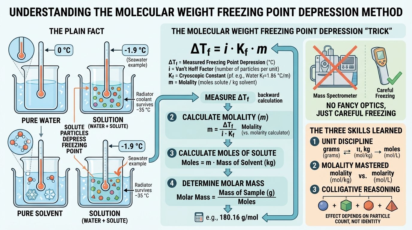
Every molecular weight freezing point depression story starts with a plain fact: pure water freezes at 0 °C. Seawater freezes near −1.9 °C. Radiator coolant survives −35 °C. The difference is dissolved particles: any solute lowers a solvent’s freezing point, and it does so in proportion to how many particles are dissolved — not what they are. This is the depression half of the molecular weight freezing point depression method, one of the four colligative properties, and it obeys a beautifully simple law: ΔTf = i · Kf · m, where m is the molality (moles of solute per kilogram of solvent), Kf is a constant belonging to the solvent, and i counts the particles each formula unit releases.
The molecular weight freezing point depression connection comes from reading that law backwards. ΔTf tells you the molality; the molality and the solvent mass tell you the moles; and moles under a weighed sample tell you the molar mass. One thermometer measurement — the whole molecular weight freezing point depression trick — converts grams into a molecular weight — no mass spectrometer, no fancy optics, just careful freezing.
That inversion made the molecular weight freezing point depression technique the dominant molar-mass method for nearly a century, and it remains a fixture of every physical and general chemistry course because it teaches three skills at once: molality (as opposed to the molarity our molarity calculator handles), colligative reasoning, and unit discipline. The calculator above runs the arithmetic in both directions — unknown to molar mass, and formula to predicted freezing point — with molar masses drawn from the same IUPAC data as our molecular weight calculator homepage.
How to Use This Calculator
Solving a molecular weight freezing point depression problem takes under ten seconds:
- Pick a molecular weight freezing point depression mode from the five tabs — Molar Mass from ΔTf, ΔTf & New FP, Van ‘t Hoff (i), Antifreeze Dose, or Molar Mass from ΔTb.
- Enter your data — sample and solvent masses with the measured ΔTf and Kf, or a solute formula with one of the seven built-in solvents. The preset chips load classic textbook setups in one click.
- Press the blue button (or hit Enter). The answer appears with the molality, the moles, a full data table and an animated comparison graph.
- Read the molecular weight freezing point depression extras — the boiling-point bonus in Mode 2, the dissociation verdict in Mode 3, or the gram-dose in Mode 4.
- Copy, download or share the result — CSV, TXT, print, WhatsApp, Facebook or X — and press ↺ Reset to start the next problem clean.
Your last ten calculations are saved in the history panel under the tool (stored only in your own browser), and Clear All wipes them instantly. Nothing is sent to any server — the entire molecular weight freezing point depression calculator runs on your device, which is also why it loads fast and works offline once the page is open.
The Five Modes Explained
🧊 Mode 1 — Molar Mass from ΔTf
The headline molecular weight freezing point depression experiment: sample mass, solvent mass, measured drop, Kf — and out comes the molar mass via M = i·Kf·w·1000 ÷ (ΔTf·W). The classic benzene unknown (1.25 g, 20.0 g, 1.02 °C) returns 313.73 g/mol with molality and moles alongside.
❄️ Mode 2 — ΔTf & the New Freezing Point
The forward molecular weight freezing point depression direction: type a solute formula (parentheses and hydrates work), the masses, pick a solvent — the mode computes the molar mass from IUPAC 2021 atomic weights, the molality, ΔTf and the new freezing point, plus the boiling-point elevation as a bonus. Ten grams of glucose in 100 g of water: ΔTf = 1.0324 °C, freezes at −1.03 °C, boils at 100.28 °C.
🧂 Mode 3 — Van ‘t Hoff Factor (i)
Electrolytes overshoot every molecular weight freezing point depression prediction: 0.1 molal NaCl should depress water by 0.186 °C as a nonelectrolyte, but measures 0.347 °C. This mode extracts i = ΔTf ÷ (Kf·m) = 1.866 and, given the expected ion count, the apparent dissociation (86.6%) — with a verdict explaining ion pairing.
🚗 Mode 4 — Antifreeze Dose
The molecular weight freezing point depression law worked backwards: pick a target freezing point and the mode returns the required molality and grams. Protecting one kilogram of water down to −10 °C takes 333.7 g of ethylene glycol — computed in two lines, and refused politely if you ask for a target above the solvent’s normal freezing point.
🌡️ Mode 5 — Molar Mass from ΔTb
The molecular weight freezing point depression method’s mirror, ebullioscopy: ΔTb = Kb·m gives the same molar mass from the boiling side — M = Kb·w·1000 ÷ (ΔTb·W). Since Kb values are smaller (water’s is just 0.512), the drops are subtler; use it to cross-check a cryoscopy result, exactly as classical labs did.
The Formula (With the Box You Should Memorize)
Every molecular weight freezing point depression problem — no exceptions — is one of these three lines rearranged:
ΔTf = i · Kf · m (m = mol solute ÷ kg solvent)
M = i · Kf · wsolute · 1000 ÷ (ΔTf · wsolvent)
ΔTb = i · Kb · m · new FP = FPpure − ΔTf · i = ΔTf ÷ (Kf · m)
Kf: water 1.86 · benzene 5.12 · cyclohexane 20.0 · camphor 39.7 °C·kg/mol · i = 1 for nonelectrolytes
Two details in that molecular weight freezing point depression box decide most marks. First, molality, not molarity: colligative laws count particles per kilogram of solvent, because kilograms don’t shrink when the solution cools. The 1000 in the molecular weight freezing point depression formula is just the grams-to-kilograms conversion for the solvent mass. Second, ΔTf is a magnitude: it’s how far the freezing point falls, always positive in the formula; the new freezing point is the pure solvent’s value minus ΔTf.
Notice also what the molecular weight freezing point depression formula rewards: a big Kf. Water’s modest 1.86 means a 313 g/mol unknown at typical concentrations moves the freezing point by barely 0.1 °C — hard to read on a thermometer. Benzene’s 5.12 triples the signal, and camphor’s colossal 39.7 amplifies it twentyfold, which is exactly why the Rast method dissolved unknowns in molten camphor and read the depression with an ordinary thermometer.
Why It Works: Colligative Properties
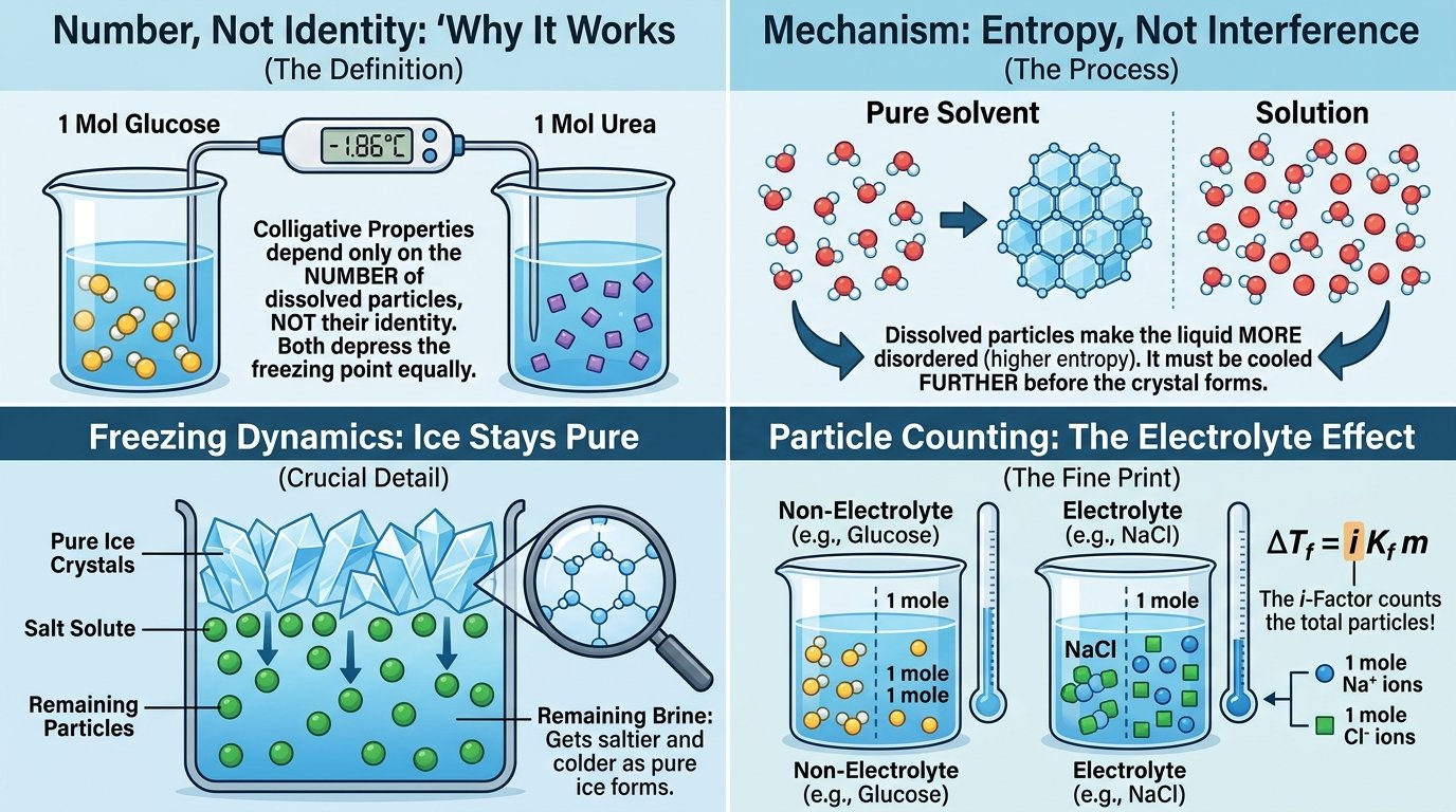
The molecular weight freezing point depression method belongs to a family of four — vapor-pressure lowering, boiling-point elevation, freezing-point depression and osmotic pressure — called colligative properties, from the Latin colligatus, “bound together.” What binds them is indifference: they depend on the number of dissolved particles, not their identity. A mole of glucose and a mole of urea depress water’s freezing point identically, despite having nothing chemically in common.
The mechanism behind every molecular weight freezing point depression measurement is entropy, not interference. Freezing requires solvent molecules to leave a disordered liquid for an ordered crystal. Dissolved particles make the liquid more disordered — more entropically comfortable — so the solvent must be cooled further before the crystal becomes worth joining. Crucially, the solute stays out of the growing ice: the crystal that forms is pure solvent, which is why sea ice is drinkable once melted and why the remaining brine gets saltier and colder as freezing proceeds.
Particle-counting is also the molecular weight freezing point depression fine print. The law is exact only in the dilute limit; concentrated solutions deviate as particles start interacting. And “number of particles” is precisely where electrolytes cause drama — the subject of the next section, and the reason the i sits in front of every formula on this page. It’s the same headcount logic that runs our average molecular weight of mixture guide, applied to a thermometer instead of a mixture.
Electrolytes and the Van ‘t Hoff Factor
Run the baseline molecular weight freezing point depression check: dissolve 0.1 mol of sucrose in a kilogram of water and the freezing point drops 0.186 °C — exactly Kf × m. Dissolve 0.1 mol of NaCl and it drops 0.347 °C, nearly twice as much. The salt has split into Na⁺ and Cl⁻, and the thermometer counts both. The van ‘t Hoff factor i captures this: i = 1 for nonelectrolytes, approaching 2 for NaCl, 3 for CaCl₂, 4 for AlCl₃ — approaching, never quite reaching.
The shortfall is the interesting part of molecular weight freezing point depression data. NaCl’s measured i of 1.87 (not 2.00) at 0.1 molal doesn’t mean 13% of the salt failed to dissolve — it means oppositely charged ions occasionally travel as paired couples, momentarily counting as one particle. Ion pairing grows with concentration and with charge: CaCl₂ manages i ≈ 2.7 out of an ideal 3, and MgSO₄, with its doubly charged pair, limps along near 1.2. Mode 3 turns any measurement into i and an apparent dissociation percentage, with the verdict spelled out.
For molecular weight freezing point depression work the practical rule is simple: determining an unknown’s molar mass assumes i = 1, so use nonelectrolyte solutes or non-dissociating solvents (benzene, camphor). Conversely, if you already know the formula — say from our formula weight calculator — a measured ΔTf becomes a probe of how completely the compound dissociates. One law, two instruments.
Three Worked Examples, Step by Step
Example 1 — The classic molecular weight freezing point depression problem
Step 1. Molality: m = ΔTf ÷ Kf = 1.02 ÷ 5.12 = 0.19922 mol/kg.
Step 2. Moles: n = 0.19922 × 0.0200 kg = 0.0039844 mol.
Step 3. Molar mass: M = 1.25 ÷ 0.0039844 = 313.73 g/mol.
Example 2 — Predicting a freezing point from a formula
Step 1. Moles: 10 ÷ 180.156 = 0.05551 mol; molality = 0.05551 ÷ 0.100 kg = 0.5551 mol/kg.
Step 2. ΔTf = 1.86 × 0.5551 = 1.0324 °C → the solution freezes at −1.03 °C.
Bonus. ΔTb = 0.512 × 0.5551 = 0.284 °C → it boils at 100.28 °C. Both ends move; freezing moves more.
Example 3 — An electrolyte’s van ‘t Hoff factor
Step 1. Ideal (i = 1) depression: 1.86 × 0.100 = 0.186 °C.
Step 2. i = 0.347 ÷ 0.186 = 1.866.
Step 3. Apparent dissociation: α = (1.866 − 1) ÷ (2 − 1) = 86.6% — the shortfall is ion pairing, not undissolved salt.
Run all three in the free calculator above and compare its printed steps with these — they match line for line, because the tool executes exactly this arithmetic at full precision.
Reference Table: Kf and Kb for 7 Solvents
The solvent sets the sensitivity of every molecular weight freezing point depression measurement. These are the seven built into the calculator:
| Solvent | Kf (°C·kg/mol) | Freezing point (°C) | Kb (°C·kg/mol) | Boiling point (°C) |
|---|---|---|---|---|
| Water | 1.86 | 0.00 | 0.512 | 100.0 |
| Benzene | 5.12 | 5.50 | 2.53 | 80.1 |
| Cyclohexane | 20.0 | 6.50 | 2.79 | 80.7 |
| Camphor | 39.7 | 178.4 | 5.95 | 204.0 |
| Acetic acid | 3.90 | 16.60 | 3.07 | 118.1 |
| Naphthalene | 6.94 | 80.20 | 5.80 | 218.0 |
| Chloroform | 4.68 | −63.5 | 3.63 | 61.2 |
Read the Kf column as the molecular weight freezing point depression sensitivity dial. The same 0.1 molal solution moves water’s freezing point by 0.19 °C, benzene’s by 0.51, cyclohexane’s by 2.0 and camphor’s by nearly 4 °C — a signal anyone can read on a school thermometer. Note also that every solvent’s Kf beats its Kb: freezing responds more than boiling, which is why cryoscopy beat ebullioscopy historically. Hydrated solutes deserve care here — dissolve CuSO₄·5H₂O and the water of crystallization joins the solvent; our molar mass of hydrates calculator covers that bookkeeping.
Running the Experiment Well
The arithmetic is the easy 10% of molecular weight freezing point depression work — the measurement is where molecular weight freezing point depression experiments earn their error bars:
- Cooling curves, not single readings — the heart of molecular weight freezing point depression technique: — record temperature versus time; the freezing point is the plateau (pure solvent) or the inflection where crystals appear (solution).
- Beat supercooling — solutions routinely dip below their true freezing point before crystallizing; seed with a crystal or scratch the vessel wall, and read the plateau after the recovery spike, not the minimum.
- Use a Beckmann thermometer or thermistor — the classical instrument resolves 0.001 °C over a 5-degree window; modern digital probes do the same with less mercury.
- Stir constantly — temperature gradients fake plateaus; gentle steady stirring keeps the reading honest.
- Stay dilute — the law is a dilute-solution limit; keep molality below ~0.5 for water (higher in high-Kf solvents where signals are already big).
- Mind volatile or associating solutes — acetic acid dimerizes in benzene (apparent M doubles!), and solutes that evaporate change concentration mid-run. Anomalous results are often chemistry, not error.
That dimerization footnote is a classic molecular weight freezing point depression exam twist: benzoic acid in benzene returns roughly twice its formula weight because hydrogen-bonded pairs count as single particles. The thermometer never lies — it just counts particles you didn’t know you had.
Who Uses the Freezing Point Depression Method?
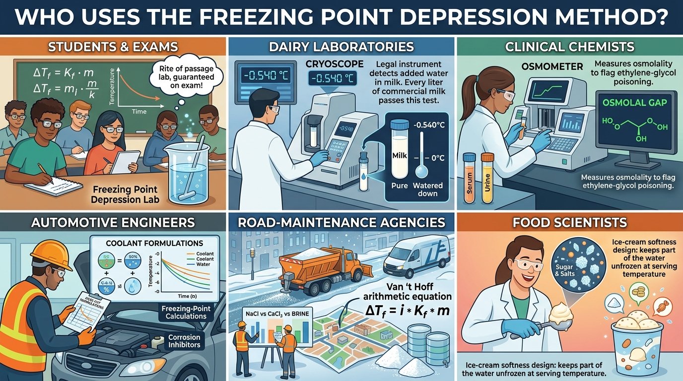
- Students — the molecular weight freezing point depression problem is a guaranteed fixture of general and physical chemistry exams, and the lab itself is a rite of passage.
- Dairy laboratories — the cryoscope is a legal instrument: milk freezes at −0.540 °C, and any drift toward 0 °C reveals added water. Every liter of commercial milk passes this test.
- Clinical chemists — freezing-point osmometers measure serum and urine osmolality, flagging the “osmolal gap” that betrays ethylene-glycol poisoning.
- Automotive engineers — coolant formulations are freezing-point calculations with corrosion inhibitors on top.
- Road-maintenance agencies — choosing NaCl vs CaCl₂ vs brine pre-treatment is applied van ‘t Hoff arithmetic at municipal scale.
- Food scientists — ice-cream softness is a freezing-point-depression design problem: sugars and salts keep part of the water unfrozen at serving temperature.
For the reaction-side math these labs run next — yields, limiting reagents, conversions — our stoichiometry calculator and grams to moles calculator continue the workflow.
Full Lab Walkthrough: An Unknown in Benzene
Here’s a complete molecular weight freezing point depression determination, exactly as the teaching lab runs it.
The task: a molecular weight freezing point depression identification of an unknown organic solid believed to be either naphthalene (128.2), biphenyl (154.2) or triphenylmethane (244.3).
- Calibrate. Freeze 20.00 g of pure benzene three times: plateau at 5.50 °C, reproducible to ±0.01.
- Dissolve. Add 0.4820 g of the unknown; record the cooling curve; crystals now appear at 4.26 °C — ΔTf = 1.24 °C.
- Compute with the molecular weight freezing point depression calculator. Mode 1: 0.482 g, 20.0 g, 1.24 °C, Kf 5.12 → m = 0.24219 mol/kg, n = 0.0048438 mol, M = 99.5 g/mol… which matches none of the candidates.
- Diagnose. Supercooling! The 4.26 °C reading was the dip, not the plateau. Re-reading the curve’s recovery gives 4.52 °C → ΔTf = 0.98 °C.
- Recompute. M = 5.12 × 0.482 × 1000 ÷ (0.98 × 20) = 125.9 g/mol — naphthalene, within 2% of 128.2.
- Cross-check. Mode 5 with a quick ebullioscopy run (ΔTb 0.505 °C for 1.28 g in 50 g) returns 128.25 g/mol. Confirmed; report printed from the toolbar.
The molecular weight freezing point depression lesson the numbers teach: the arithmetic was never the risk — the supercooled reading was. Verify the curve, then trust the calculator.
A Short History: Blagden, Raoult & the Rast Method
The molecular weight freezing point depression law came before its theory. In 1788 Charles Blagden, secretary of the Royal Society, showed that salt lowers water’s freezing point in proportion to the amount dissolved — Blagden’s law, a century ahead of its explanation. The explanation arrived with François-Marie Raoult in 1880s Grenoble, who measured depressions for dozens of solutes with monastic patience and found the constant-per-mole regularity that turned a curiosity into an instrument: if equal moles give equal depressions, then an unknown’s ΔTf reveals its moles, and hence its molecular weight.
Molecular weight freezing point depression measurements promptly changed chemistry. It was how the molar masses of countless organics were first pinned down, how Beckmann’s 0.001-degree thermometer became standard glassware, and how van ‘t Hoff — armed with the anomalous factors of electrolytes — built the case for ions in solution that earned the first Nobel Prize in Chemistry in 1901 (and Arrhenius his in 1903). Karl Rast’s 1922 trick of using molten camphor (Kf ≈ 40) let chemists determine molecular weights with milligram samples and ordinary thermometers. Mass spectrometry eventually took the crown for precision — the story our monoisotopic mass calculator tells — but the freezing point method still delivers molar masses with equipment a school owns, which is why it never left the syllabus.
Freezing Point Depression in Everyday Life
- Road salt — NaCl brine works to about −9 °C practically; below that, crews switch to CaCl₂ (i ≈ 3, and it releases heat while dissolving).
- Car antifreeze — a 50:50 ethylene-glycol mix protects to roughly −37 °C; the same jug raises the boiling point for summer, both ends of the colligative law in one product.
- Homemade ice cream — salt on ice pulls the brine below −10 °C, cold enough to freeze the custard; the sugar inside the custard keeps it scoopable.
- Seawater — 3.5% salt depresses the ocean’s freezing point to −1.9 °C; sea ice that forms is nearly fresh, concentrating brine below.
- Antifreeze in nature — Arctic fish, overwintering insects and frost-tolerant plants load their fluids with glycerol, sugars and antifreeze proteins.
- De-icing aircraft — propylene-glycol sprays are a calculated dose against the forecast, Mode 4 at airport scale.
- Freezer-proof vodka — 40% ethanol depresses the freezing point to about −27 °C, which is why the bottle pours straight from the freezer.
Every bullet is the same molecular weight freezing point depression law wearing different clothes — particles in a solvent, counted by a thermometer.
Practice Problems (With Answers)
Work each problem by hand first, then verify with the free calculator above. Answers are hidden until you click.
Problem 1 — 5.00 g of a nonelectrolyte in 100 g of water freezes at −0.516 °C. Find M.
m = 0.516 ÷ 1.86 = 0.27742 mol/kg → n = 0.027742 mol → M = 5.00 ÷ 0.027742 = 180.23 g/mol — consistent with glucose.
Problem 2 — What does 62 g of ethylene glycol (C₂H₆O₂) in 250 g of water freeze at?
M = 62.068 → 0.9989 mol → m = 3.9956 mol/kg → ΔTf = 1.86 × 3.9956 = 7.4318 °C → freezes at −7.43 °C.
Problem 3 — 0.100 molal CaCl₂ in water measures ΔTf = 0.50 °C. Find i and the apparent dissociation.
i = 0.50 ÷ (1.86 × 0.100) = 2.688; α = (2.688 − 1) ÷ (3 − 1) = 84.4% — ion pairing accounts for the rest.
Problem 4 — How many grams of sucrose (C₁₂H₂₂O₁₁, M = 342.297) bring 500 g of water to −2.00 °C?
m = 2.00 ÷ 1.86 = 1.07527 mol/kg → n = 0.53763 mol → grams = 0.53763 × 342.297 = 184.03 g.
Problem 5 — 1.28 g of an unknown in 50 g of benzene raises the boiling point by 0.505 °C (Kb = 2.53). Find M.
M = 2.53 × 1.28 × 1000 ÷ (0.505 × 50) = 128.25 g/mol — naphthalene, cross-checked from the boiling side.
Tips for Fast, Error-Free Calculations
- ✅ Convert the solvent to kilograms first — the number-one molecular weight freezing point depression habit: — the 1000 in the formula exists only because solvent masses arrive in grams; do it explicitly and the units audit themselves.
- ✅ Keep ΔTf positive — it’s the size of the drop; subtract from the pure freezing point only at the very end.
- ✅ Molality, never molarity — kilograms of solvent, not liters of solution; the whole law depends on it.
- ✅ Check i before you start — nonelectrolyte? i = 1 and vanishes. Salt? Count the ions and expect a little less (ion pairing).
- ✅ Sanity-check every molecular weight freezing point depression result against a candidate formula — a cryoscopic 313.7 g/mol with 2% error brackets 308–320; compare candidates before celebrating.
- ✅ Reset between problems — the ↺ Reset button on each mode keeps old inputs from contaminating the next calculation.
⚗️ Pro workflow: Mode 1 for any molecular weight freezing point depression unknown → Mode 2 to predict a freezing point before mixing → Mode 3 when the solute is an electrolyte → Mode 4 to dose antifreeze or road salt → Mode 5 to confirm from the boiling side. Five tabs, one colligative law, zero unit slips.
5 Common Mistakes to Avoid
A decade of marking molecular weight freezing point depression answers produces the same five errors on repeat:
- Using molarity instead of molality in molecular weight freezing point depression work. Liters of solution ≠ kilograms of solvent; in dilute water they’re close enough to almost work, which makes the habit dangerous everywhere else.
- Forgetting the 1000. Solvent grams must become kilograms; omitting the factor makes every molar mass a thousand times too small — instantly recognizable, still endlessly submitted.
- Dropping the van ‘t Hoff factor. For NaCl solutions every prediction is nearly double without i — and conversely, using i on a nonelectrolyte halves it.
- Reading the supercooled minimum as the freezing point. The classic molecular weight freezing point depression trap: The plateau after recovery is the true value; the dip can be half a degree low, wrecking the molar mass.
- Confusing ΔTf with the new freezing point. ΔTf = 1.03 °C means the solution freezes at −1.03 °C (for water), not +1.03 — signs belong to the last step only.
How This Calculator Is Different
| Feature | This calculator | Generic ΔTf tool | By hand |
|---|---|---|---|
| Molar mass from ΔTf (the inverse problem) | ✅ With molality & moles shown | ⚠️ Forward only | ✅ If units survive |
| Formula input (IUPAC 2021 masses) | ✅ Parentheses & hydrates | ❌ Numbers only | ⚠️ Separate lookup |
| Van ‘t Hoff factor & dissociation verdicts | ✅ i and α with interpretation | ❌ | ✅ If you know the trick |
| Antifreeze dose (inverse to grams) | ✅ With target-FP validation | ❌ | ⚠️ Two rearrangements |
| Ebullioscopy cross-check | ✅ Same interface, Kb built in | ❌ | ⚠️ Rare |
| Export & history | ✅ CSV/TXT/print/share + last 10 | ❌ Usually none | ❌ Notebook |
Related molecular weight freezing point depression companions carry the theme onward: exact and isotope-level masses in the exact mass calculator, isotopic mass calculator and average vs monoisotopic mass guide — and the polymer-scale averages this method historically fed into, via the number average molecular weight polymer, weight average molecular weight polymer and polydispersity index calculator trilogy (cryoscopy measures a number-average, incidentally — every particle votes once).
Where the Numbers Come From
The Kf and Kb constants built into this molecular weight freezing point depression calculator are the standard literature values used by mainstream physical-chemistry texts (water 1.86/0.512, benzene 5.12/2.53, cyclohexane 20.0/2.79, camphor 39.7, acetic acid 3.90/3.07, naphthalene 6.94, chloroform 4.68/3.63 °C·kg/mol). Molar masses computed from formulas use IUPAC 2021 standard atomic weights — the same 118-element dataset behind every tool on this site. The atomic mass calculator exposes that dataset element by element.
Molecular weight freezing point depression textbooks differ slightly on some constants (camphor appears as 37.7–40.0 depending on purity and source) — if your course sheet specifies a value, type it directly into Modes 1, 3 or 5. Spot a discrepancy worth checking? Our corrections policy explains how we verify and fix reports — usually within days.
Exam Checklist
☐ I can rearrange it to M = i·Kf·w·1000 ÷ (ΔTf·W) without notes.
☐ I know Kf for water (1.86) and benzene (5.12), and why camphor’s 39.7 made the Rast method work.
☐ I can convert ΔTf into a new freezing point with the correct sign.
☐ I can compute a van ‘t Hoff factor from data and interpret i < n as ion pairing.
☐ I can explain why colligative properties count particles, not identities.
☐ I know the classic traps: supercooling, dimerization in benzene, molarity vs molality.
☐ I’ve verified my practice answers with the molecular weight freezing point depression calculator above.
Frequently Asked Questions
How do you find molecular weight by freezing point depression?
Dissolve a weighed sample (w grams) in a weighed solvent (W grams), measure the drop ΔTf, and apply M = Kf × w × 1000 ÷ (ΔTf × W). Example: 1.25 g in 20.0 g benzene with ΔTf = 1.02 °C gives M = 313.73 g/mol.
What is the freezing point depression formula?
ΔTf = i · Kf · m, where m is molality (mol solute per kg solvent), Kf is the solvent’s cryoscopic constant and i is the van ‘t Hoff factor (1 for nonelectrolytes). The new freezing point is the pure solvent’s minus ΔTf.
Why molality and not molarity?
Because volumes change with temperature but masses don’t. A solution cooled toward freezing contracts, so mol/L would drift mid-experiment; mol/kg stays fixed, which is why every colligative law uses it.
What is Kf for water?
1.86 °C·kg/mol — one mole of dissolved particles per kilogram of water lowers the freezing point by 1.86 °C. Benzene’s is 5.12, cyclohexane’s 20.0 and camphor’s 39.7, which is why high-Kf solvents make more sensitive measurements.
Is this molecular weight freezing point depression calculator free?
Yes, completely free — no registration, no daily limits. It runs entirely in your browser, and your history stays on your own device.
What is the van ‘t Hoff factor?
The effective number of particles each formula unit releases: 1 for sugar, ~1.9 for NaCl, ~2.7 for CaCl₂ at ordinary concentrations. Measured i values fall short of the ideal ion count because of ion pairing; Mode 3 computes both i and the apparent dissociation.
Why does salt melt ice on roads?
Salt dissolving into the thin water film lowers its freezing point below the ambient temperature, so ice keeps melting instead of re-freezing. NaCl works to about −9 °C in practice; CaCl₂ (three ions, plus heat of dissolution) reaches −20 °C and below.
What was the Rast method?
Karl Rast’s 1922 micro-technique using molten camphor as the solvent. Camphor’s huge Kf (≈ 39.7) turns tiny molalities into several-degree depressions, so molecular weights could be measured with milligram samples and an ordinary thermometer.
Why did my benzoic acid come out at double its molar mass?
Carboxylic acids dimerize in benzene through hydrogen bonding, so two molecules travel as one particle — the thermometer counts half the expected particles and the computed M doubles. It’s the classic “anomalous molecular weight” exam question.
Can freezing point depression measure polymers?
Only small ones. A 100,000 g/mol polymer at practical concentrations produces depressions of a few ten-thousandths of a degree — unmeasurable. Historically cryoscopy handled oligomers; large polymers went to osmometry and light scattering, which report the averages covered in our polymer calculators.
10 Cryoscopy Facts Worth Knowing
- Blagden’s law (1788) preceded its own explanation by almost exactly a century — Raoult systematized it in the 1880s.
- Van ‘t Hoff’s analysis of “anomalous” electrolyte depressions helped win the very first Nobel Prize in Chemistry, in 1901.
- The Beckmann thermometer, invented for cryoscopy, reads 0.001 °C — over a window of only about 5 degrees, set by sliding mercury between reservoirs.
- Milk’s freezing point (−0.540 °C) is so reproducible that cryoscopes are legal instruments for detecting watered-down milk worldwide.
- Clinical osmometers use freezing point depression to screen for ethylene-glycol poisoning — the “osmolal gap” appears hours before lab confirmation.
- Sea ice is nearly fresh: the crystal excludes salt, which is why melted multi-year ice is drinkable and the brine beneath grows denser.
- A 50:50 glycol-water mix doesn’t obey the dilute law (it’s hardly dilute) — real coolant charts are measured, not calculated, but the law still sets the trend.
- Camphor’s Kf ≈ 39.7 is about 21× water’s — the entire trick behind Rast’s milligram-scale molecular weights.
- Cryoscopy yields a number-average molecular weight: every particle votes once, exactly like the polymer Mn our tools compute.
- Antifreeze proteins in polar fish work differently — they bind ice crystals and block growth, achieving “thermal hysteresis” far beyond their colligative share.
🔗 Trusted external resources
Final Thoughts
The molecular weight freezing point depression method is a rare thing in chemistry: a molecular measurement you can make with kitchen-grade equipment and one careful thermometer. Behind it sit four small rules — molality not molarity, ΔTf as a positive magnitude, the 1000 that converts grams to kilograms, and an i for every electrolyte. Master those, let the calculator above verify every line, and cryoscopy becomes one of the most dependable places to score — in the exam hall and at the bench.
Bookmark this molecular weight freezing point depression page for your next problem set or lab report, share it with a labmate before the cryoscopy practical, and explore the rest of our free chemistry tools — from the molecular weight calculator homepage to the molarity calculator for the solution-prep side. Questions or corrections? Reach us any time through the contact page — and you can read more about the site’s mission on our about page.
Written & Reviewed By
Ahmad Raza, M.Phil. Chemistry
Ahmad is a chemistry educator and science content developer with over 10 years of experience teaching analytical and physical chemistry. He builds free calculation tools that help students and lab professionals work faster and make fewer errors. When he’s not balancing equations, he’s usually grading titration reports.